Overview of Interactive Modeling

Adding Interactive Modeling to the Pipeline

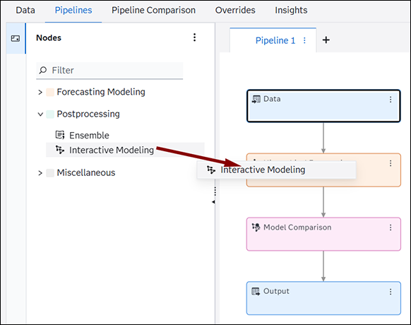
The Interactive Modeling node is listed in the Nodes pane on the left under Postprocessing. It can be added to a pipeline using one of these methods:

• Drag the node to the pipeline and place it over a modeling node.
  
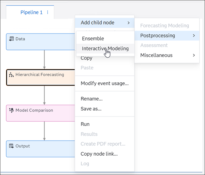
• Right-click the modeling node and select Add child nodePostprocessingInteractive Modeling.
  

After you add Interactive Modeling, the pipeline shows a connection from the modeling node to Interactive Modeling and Model Comparison. You can connect other modeling nodes and any Ensemble nodes to an Interactive Modeling node.

You cannot add an Interactive Modeling node to an External Forecast pipeline.

Adding Multiple Modeling Nodes to Interactive Modeling Node

You can add multiple modeling nodes to a single Interactive Modeling node. When the pipeline is run, the Interactive Modeling node evaluates the performance of each preceding node and assigns the champion model for each time series based on the model selection criteria chosen for the Interactive Modeling node. Follow these steps to add other modeling nodes to Interactive Modeling.

1. Right-click the Interactive Modeling node and choose Select Models.

   Modeling nodes that are available in the pipeline are listed in the menu.

   

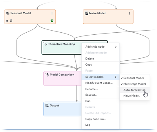
2. Select any modeling node that you want to add. If modeling nodes are connected to an Ensemble node, they are also available in the list to be connected to this Interactive Modeling node.

   Deselect any modeling node that you want to remove.

3. Run the pipeline again to see the new results.

Options

The following options are available in the right pane of the Pipelines tab when Interactive Modeling is selected.

Reapply champion selection after the node is re-run

This option is used to preserve any selected champion models that you save to the Interactive Modeling node in case future updates invalidate the pipeline. Project changes can include refreshing the project data or changing the project settings. For a complete list, see Changes That Invalidate Pipelines.

After the pipeline is invalidated, run the pipeline again. If Reapply champion selection after the node is re-run is not checked, then any models that you have selected and saved as champions are no longer designated as champions. For more information, see Selecting a Different Champion Model.

Note: This option has no effect if a change is made to the project hierarchythe order of the variables that you have assigned to the BY variables role. An example of a hierarchy is Region > Product Category > Product Line. . Adding, removing, or changing the position of a BY variable in the hierarchy removes any custom models from the Model Selection List table. It also removes any champion model designations that have been saved in the Model Selection List. The custom models can be restored by returning the project hierarchy to its original state.

Inherit model selection list of predecessor modeling node

Select this option to include all of the candidate models from each predecessor modeling node. If you choose this option, the Modeling tab shows a list of models from each predecessor, but only if you select the Forecast model selection graph as an output table from the predecessor. Interactive Modeling can inherit the model selection lists only from these modeling nodes:

• Auto-forecasting
• Naive Model
• Seasonal Model
• Non-seasonal Model

For more information about how this works, see Modeling Tab.

Also, see Selected Champion Model Is Removed from Interactive Modeling for further information.

Automatic Forecast Selection

The options in this section determine how the champion model is selected for each time series. Interactive Modeling selects the best performing modeling node as the champion.

Specify criterion

Select the statistic of fita statistical value that is used to evaluate how well a forecasting model fits the historical series by comparing the actual data to the predicted values. that you want to use to determine the default champion modeling for each time series. This default champion can be one of the predecessor nodes or a custom model if you decide to include custom models in automatic forecasta numerical prediction of a future value for a specified time period for each unique combination of BY variable values selection. The default is RMSE.

Include

The predecessor nodes are included in the selection for the default champion model for each time series. Select Custom models if they should also be candidates for the default champion model selection.

Default champion models are identified only when Interactive Modeling is run from the pipeline. Therefore, after new custom models are added to time series or existing custom models are edited within Interactive Modeling, you must run the node again so that they can be evaluated for default champion status. You can also select custom models as champion when you are working within Interactive Modeling.

Model suggestions

The following models are selected by default to be evaluated for the best fit for each time series. You can deselect any of them if you do not want them included in Interactive Modeling.

• Include ESM models
• Include ARIMAX models
• Include IDM models

Note: If no model can be fit based on the selected models, the DIAG_ESMBEST_DEFAULT model is fit to the time series.

You can use the following options to select the best model within each predecessor node.

• IDM Settings

  Sensitivity level for intermittency test

  Specify an integer greater than one. This setting is used to determine whether a time series is intermittent. If the demand interval is equal to or greater than this number, then the series is assumed to be intermittent.

  IDM method

  Select one of the following models:

  • Average : requests the extended sample autocorrelation function.
  • Best : uses the single smoothing model to fit the average demand component.
  • Croston : uses the two smoothing models to fit the demand interval component and the demand size component.

• Number of data points used in the holdout sample

  Enter a positive integer to be used as the size of the holdout samplethe number of periods of the most recent data that should be excluded from the parameter estimation. The holdout sample can be used to evaluate the forecasting performance of a candidate model.. The actual holdout sample is the minimum between this value and the Percentage of data points used in the holdout sample . The default value is zero, which means no holdout sample is used.

• Percentage of data points used in the holdout sample

  Enter a value between 0 and 100 to specify the percentage of the sample that is used for the holdout sample. The actual holdout sample is the minimum between this value and the Number of data points used in the holdout sample . This option is displayed only if Number of data points used in the holdout sample is greater than zero.

• Model selection criterion

  Choose the statistics of fit to use when diagnosing each time series to create system-generated model suggestions on the Modeling tab of Interactive Modeling.

  For descriptions of each option, see Descriptions of Model Selection Criteria.

Hierarchical Modeling

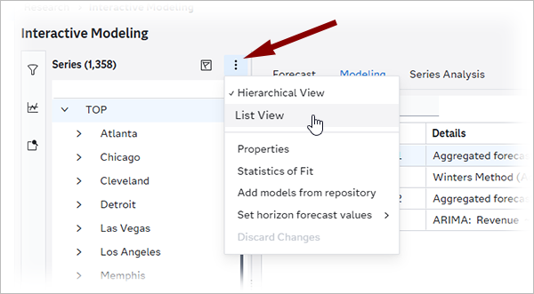
Enables you to navigate the time series in Interactive Modeling using a hierarchical tree view. This creates a tree view of the hierarchy in the Series tab, starting at the top level. You can expand and collapse each level in the hierarchy and perform interactive modeling tasks at each level, such as creating models and assigning champions.

With this option turned on, the Filters pane is not populated and can be collapsed for better viewing. If you want to view the time series in a single list, click and select List View. The Series pane changes from the tree view to the list of time series. The Filters pane is populated on the left.

With Hierarchical Modeling turned on, the forecasts for each predecessor node are aggregated from the lowest level to the highest level. If the predecessor node is a Hierarchical Modeling or Hierarchical Forecasting node, the data is used for all levels generated by the preceding modeling node.

Unless the predecessor node is Hierarchical Modeling, SAS Visual Forecasting does not diagnose the best model for higher levels of the hierarchy. Bottom-up aggregate forecasts of the lower levels are used as the base statistical forecasts. As a result, you can see different reconciled and final forecasts when using non-hierarchical modeling nodes compared to the Hierarchical Modeling node as a predecessor.

Note: Starting in release 2025.11, if this option is turned off, any overrides that are created are removed except for overrides at the lowest level of the hierarchy.

By default, the hierarchy is reconciled based on the level specified for the BY variables on the Data tab. You can change the settings using these options:

Specify the reconciliation level

The reconciliation level is specified for this node by selecting a BY variable from the hierarchy. Consider the order of the default attributes (BY variables) defined on the Data tab. Select a variable to determine the type of reconciliation methodthe method that specifies the level in the hierarchy where the process of reconciliation starts. The following reconciliation methods are available: bottom-up method, middle-out method, and top-down method. .

• Select Top to perform top-down reconciliation.
• Select the variable at the bottom of the hierarchy to use bottom-up reconciliation. For example, if the hierarchy consists of two default variables, Location at the top and Name at the bottom, select Name to perform bottom-up reconciliation.
• You can select a variable in the middle level of the hierarchy to use middle-out reconciliation. For example, if the hierarchy consists of three default variables in the order of High, Medium, and Low (with High at the top), specify Medium to generate forecasts for that level and then reconcile forecasts for the upper and lower levels in the hierarchy.

By default, the reconciliation level set on the Data tab for the BY variables is used.

For a description of top-down, middle-out, and bottom-up reconciliation methods, see Understanding Hierarchy Reconciliation.

Disaggregation method during top-down disaggregation

specifies the type of disaggregation methoda method that specifies how the forecasts in the lower level of the hierarchy are reconciled when the reconciliation method is top-down or middle-out. The disaggregation method can reconcile the forecasts in either of the following ways: (1) by using the proportion that each lower-level forecast contributes to the higher-level forecast; or (2) by splitting equally the difference between the higher-level forecast and the lower-level forecasts. and type of loss function for top-down reconciliation. Select one of the following methods for top-down disaggregation:

• Difference — bases the loss function on the root mean square error (RMSE). This results in adjustments that are the (possibly weighted) mean difference of the aggregated child nodes and the parent node.
• Proportions — uses a loss function that results in reconciled forecasts that are the (possibly weighted) proportional disaggregation of the parent node.

Output Tables

The following tables are automatically generated when running Interactive Modeling. After the node is run, the tables can be saved using the Save Data Node.

• Statistics of Fit (OUTSTAT)
• Descriptive Statistics (OUTSUM)
• User-Defined and Derived Attributes (MERGED_ATTRIBUTES)
• Weights of Constituent Nodes (OUTWEIGHT)
• Forecasted Values (OUTFOR)

The following tables are optional.

• Parameter Estimates (OUTEST)
• Model Forecast Components (OUTCOMPONENT)

See Results for more information about how these tables are processed.

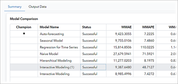
Results

The Interactive Modeling node does not have a results page that is similar to what the modeling nodes provide (that shows the MAPE distribution and execution summary). However, when the Interactive Model is the champion node of the pipeline, you can view the output tables that it updates through the Results viewer of the Model Comparison node. The Interactive Modeling node updates the following tables when these tables are produced by its immediate predecessor:

• OUTSTAT
• OUTSUM
• MERGED_ATTRIBUTES
• OUTFOR

See Also

• Model Comparison
• Save Data Node
• Parameter Estimates Table Is Missing after Upgrading to the 2024.09 Release

Content of Interactive Modeling

After this node is run, right-click the node and select Open to view the results. The Interactive Modeling node has the following layout.

Filters

By default, the left pane shows Filters , which provides a list of attributes with which you can create filtersa set of specified criteria that are applied to data in order to identify the subset of data for a subsequent operation, such as continued processing. from the project data. See Filters for more information.

If Hierarchical Modeling is turned on for this node, the Filters pane is empty. You can collapse this pane by clicking to the left.

Series

The time series are listed using each unique combination of BY variable values.

If Hierarchical Modeling is turned on, the series are arranged in a tree format starting from the top level of the hierarchy. If Hierarchical Modeling is not turned on, you can reduce the list to a smaller subset of all of the time series in the project by selecting attributes from the Filters pane.

You can change the view in the Series pane from the hierarchical tree view to a simple list of time series, as shown below.

You can select only one time series at a time. The exception to this rule is when Hierarchical Modeling is turned off and the Forecast tab is selected. In this case, you can select up to 16 time series at a time.

When you right-click a single item in the Series pane, you can select one of the following actions:

Properties

This opens a Properties window that displays some metadata about the time series, such as the starting and ending time values and the number of observations. It displays the name of the time series, which is the unique combination of BY variables that describe the time series.

Statistics of Fit

This displays a table showing the name of the time series followed by the in-sample statistic that is the criterion selected under the Automatic Forecast Selection. If the project includes an out-of-sample regionthe number of time periods before the end of the data that are removed when fitting models. After model selection, forecasts are generated in the out-of-sample region and then compared to the actual data to determine accuracy. specified, that statistic is also shown. You can click the column heading to add other statistics to the table and arrange them in any order. For more information, see Working with Tables in SAS Model Studio in SAS Visual Forecasting: Overview.

Add models from the repository

This opens a window where you can select additional models to add to the model selection list in the Modeling tab. For more information, see Adding Models from the Model Repository to a Time Series.

Set horizon forecast values

Use this action for any time series that you need to set the forecast values to zero or missing. This change affects only forecasts in the horizonthe number of intervals into the future, beyond a base date, for which analyses and predictions are made.. It does not affect forecasts in the out-of-sample region. By default, this value is set to the Statistical forecast from the current champion model.

Forecast values for all models in the model selection list are reset when you change this setting.

If you choose to set the forecast values to zero, the plot shows the zero values in the forecast region of the Historical and forecast region plot. If you choose to set the forest values to missing, the forecast region does not show any data.

After you set horizon forecast values to zero or missing, the time series is denoted with the icon , which indicates that the change must be saved. After you save your changes, the time series is shown in the Series pane with this icon: . When you are working with the horizon forecast values, any user working in the same Interactive Modeling node cannot see your changes until you save. See Saving Your Changes in Interactive Modeling for more information.

If you need to change this setting back, right-click the time series and select Set forecast horizon valuesStatistical forecast. This change must be saved again.

Starting in release 2025.11, if you set forecast values to zero or missing, any pending or saved overrides are removed after you save the changes.

Forecast, Modeling, and Series Analysis

These tabs are along the top of the right pane.

Forecast

Like the Forecast Viewer, this tab shows an envelope plot of the dependent variable for the full time range of the project data. If Hierarchical Modeling is turned on, the TOP level of the hierarchy is selected in the Series pane. If Hierarchical Modeling is not turned on, the first series is selected in the Series pane. When Interactive Modeling node is first opened, the plot shows the forecasts from the champion predecessor modeling node.

Below the plot is the Forecasts and Overrides table. Use this table and the Override Calculator to create overrides for individual time series. For more information, see Creating Overrides for a Time Series. The table is available only when one item is selected in the Series pane.

If you do not select and save new champion models for any time series, the plot shows the forecasts from the champion predecessor modeling node. For more information, see Selecting a Different Champion Model.

Modeling

This tab is displayed initially. For any selected time series, the Modeling tab lists the predecessor modeling nodes and system-generated models. The system-generated models are the candidate models that would be generated by the equivalent of an Auto-forecasting node using the default settings.

This tab is different from the Modeling tab that is available in the Forecast Viewer of some modeling nodes. See Modeling Tab for more information.

Series Analysis

This tab is used to run analyses on individual time series. The right pane shows a plot for the item selected in the Series pane. See Conducting a Series Analysis for more information.

When the Series Analysis tab is selected, you can use these icons to the left to change to these views.

• — Lists the dependent and any independent variables that are defined for the project.
• — Lists analyses that can be added to time series that have been added to the right pane.
• To switch back to Filters , click to the left of the pane.

See Conducting a Series Analysis for more information.