Creating Overrides in Interactive Modeling
This feature is introduced in release 2025.11.
Overview
On the Forecast tab in Interactive Modeling, if you select a single time seriesan aggregation of transactional data into specified time intervals and sorted according to unique combinations of the default attributes (BY variables), the Forecasts and Overrides table is displayed below the time series plot. The top row, Historical Data, shows the actual data from the historical period. The next row, Statistical Forecast, shows the forecasts during the historical period and extends the forecasta numerical prediction of a future value for a specified time period for each unique combination of BY variable values into the forecast period (horizonthe number of intervals into the future, beyond a base date, for which analyses and predictions are made.). If you scroll to where the forecasts begin, you can enter overrides for the forecasts in each time period in the Overrides row. You can enter static forecast values in the table cells as overrides. For best results, use the Override Calculator to enter your overrides.
The following icons are available in the toolbar above the Forecasts and Overrides table.
 ─ Opens the Override
Calculator. Use the calculator to add overrides to one or more time intervals
for the selected time series.
─ Opens the Override
Calculator. Use the calculator to add overrides to one or more time intervals
for the selected time series. ─ Removes an override in a table cell that is
selected
─ Removes an override in a table cell that is
selected ─ Checks for conflicts in the overrides that have been
submitted
─ Checks for conflicts in the overrides that have been
submitted
Creating Overrides for a Time Series
Any overrides that you create or edit are preserved in your work environment and are not exposed to other project users until you save the changes. When you are working with overrides, any user working in the same Interactive Modeling node cannot see your changes until you save. When you save the changes, other users are notified and the Interactive Modeling is updated with the changes. See Saving Your Changes in Interactive Modeling for more information about saving your changes.
If Hierarchical Modeling is turned off, you can create overrides for a single selected time series. If Hierarchical Modeling is turned on, you can create overrides for any level in the hierarchy. However, if this setting is subsequently turned off, any overrides that are created are removed except for overrides that were explicitly set at the lowest level of the hierarchy.
When you are working with overrides, if your browser closes unexpectedly, your unsaved changes should be saved when you log back in and reopen Interactive Modeling.
On the Overrides row, you can enter a static forecast value in the forecast region of the table. Follow these steps to use the Override Calculator.
- Click a cell in the Overrides row for a time period in the horizon.
- Click in the toolbar over the table. This opens the
Override Calculator. The time series that you selected is listed at the top. If you have already selected
a time period, it is available in the Selected time periods
field.
- Select whether you want to create an
override for Specific time periods or for a
Fixed range of time.
- To enter more than one
selected time period, click
 to add specific periods to override.
 - If you selected a fixed range of time, enter the Beginning period and the Ending period for the range.
- To enter more than one
selected time period, click
- For Adjustment, you can select the adjustment up or down based on a percentage of the value or a number of units.
- If multiple time periods are selected
for a static value, use Distribution options to specify
how the override value is distributed to the time periods.
- Split proportional
to current forecast
This option is selected only if Hierarchical Modeling is turned on for Interactive Modeling.
- Split evenly
- Assign specified value to each period
- Split proportional
to current forecast
- Click
Apply.
The values are updated in the Overrides row. The following example shows three overrides that have been created with the Override Calculator. The clock in the cell with the override value indicates that the overrides are pending.
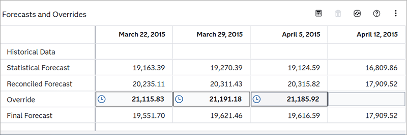
The selected time series is denoted with the icon
 , which indicates that the changes have not been saved. You are
prompted to save your changes.
, which indicates that the changes have not been saved. You are
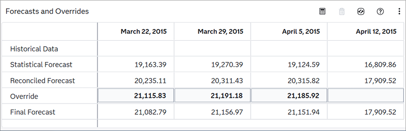
prompted to save your changes. - Click Save.
The Final Forecast row is updated with the new values based on the overrides that you entered. The clock is removed from the override values. The override value is disaggregated to the lower-level time series. The overrides have been applied.
 Note: When you click Save, if there are any override conflicts detected, the Conflict Resolution window is displayed. You must first resolve the conflicts before the changes to overrides can be saved. Conflicts can be generated only when Hierarchical Modeling is turned on for Interactive Modeling. See Working with Override Conflicts for more information.
The time series is marked with
 icon.
icon.
If you need to make changes to the override value, select the time period and open the Override Calculator to specify the new value.
See Also
Deleting Overrides
Follow these steps to delete pending or saved overrides.
- Select one or more override cells in the Forecasts and Overrides table.
- Choose one of the following
options.
- To delete only one selected
override, click .
- To delete multiple overrides,
click
 and select from the following options.
- Delete selected overrides — Deletes only the overrides that you have selected.
- Delete overrides from the selected series — Deletes all overrides in the selected series. You first have to choose between deleting only pending overrides or deleting pending and saved overrides.
- Delete overrides from all series — Deletes overrides for all time series in this Interactive Modeling node. You first have to choose between deleting only pending overrides or deleting pending and saved overrides.
- To delete only one selected
override, click
- Click Save to save your changes. If you exit Interactive Modeling without saving your changes, only the pending overrides are deleted.
Working with Override Conflicts
Resolving override conflicts is a new feature in release 2025.12.
Override conflicts are detected when you submit pending overrides or resubmit applied overrides. When you submit an override, SAS Visual Forecasting disaggregates the override value to lower-level time series. If a conflict exists, you cannot save your overrides until you resolve the conflict. Conflicts can be generated only when Hierarchical Modeling is turned on for Interactive Modeling and the project has at least one BY variable.
The following image shows the
Conflict Resolution window that opens when you try to save
overrides that have conflicts. You can also check for conflicts by clicking in the toolbar over the Forecasts and Overrides table.
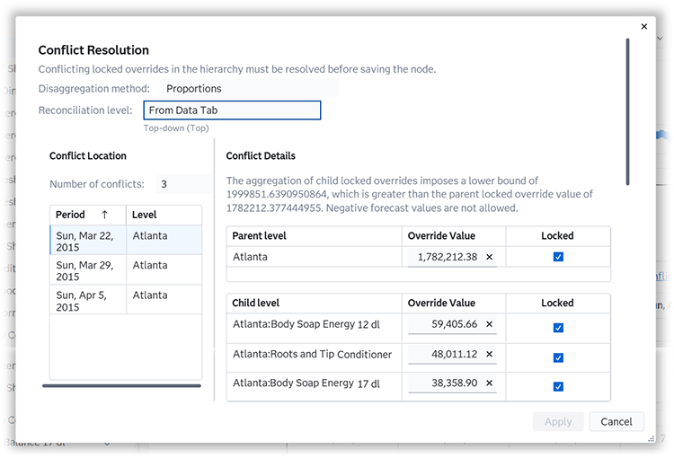
At the top, this window shows the disaggregation methoda method that specifies how the forecasts in the lower level of the hierarchy are reconciled when the reconciliation method is top-down or middle-out. The disaggregation method can reconcile the forecasts in either of the following ways: (1) by using the proportion that each lower-level forecast contributes to the higher-level forecast; or (2) by splitting equally the difference between the higher-level forecast and the lower-level forecasts. as it is defined in settings for Interactive Modeling. It also shows the reconciliation level for the Interactive Modeling node. In this figure, the reconciliation is set to use the level defined on the Data tab. Conflict Location shows the series at the parent level that conflict with the lower levels. The series are sorted by time periods.
Try one of these methods to resolve the
conflicts. While making changes, click Apply. If any conflicts
remain, they are still listed in the window. Otherwise, the window shows the message:
There are no remaining override
                  conflicts
.
- Remove the locks on some of the conflicts.
- Change the values for the overrides in the window.
- Remove overrides by clicking x next to them.
Conflicts can be generated when locked overrides are within the same time period but at different levels in the hierarchy. Negative override values, either locked or unlocked, are treated as 0 when negative forecasts are not allowed in the project.