Conducting a Series Analysis

From the Series Analysis tab in Interactive Modeling, you can display plots for any time seriesan aggregation of transactional data into specified time intervals and sorted according to unique combinations of the default attributes (BY variables) selected from the Series pane. For each time series, you can view plots for the dependent variable or any independent variable.

Overview

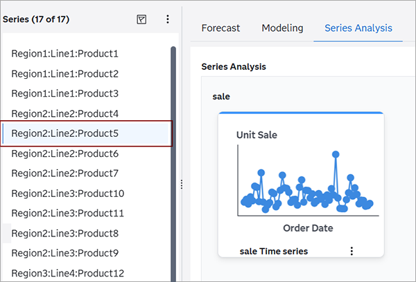
When you first select the Series Analysis tab, the right pane shows a time series plot of the dependent variable for the item that is selected in the Series pane. For time series analysis, only one item can be selected at a time.

The analyses are placed on a row for each model input. You can add more rows for each model input. If you add a model input that is already placed in the right pane, the input is added again with a number appended to the variable name. For example, if you have already placed a model input on the canvas with the name Quantity, adding it again puts the input on the canvas with this name:

Quantity (1)

For most analyses, you can add only one type for each input row. For analyses that can be modified, you can add several of these types to an input row if you change the default settings.

When you close a session in Interactive Modeling, the analyses that you have arranged are preserved for you. The next time you open Interactive Modeling and select the Series Analysis tab, the plots and graphs that you have arranged in the middle pane remain in place.

Displaying an Analysis for a Time Series

Follow these steps to display a plot for a time series.

From the Series Analysis tab in Interactive Modeling, select an item in the Series pane.
The plot for the selected time series is generated and displayed on the canvas in the Series Analysis tab.

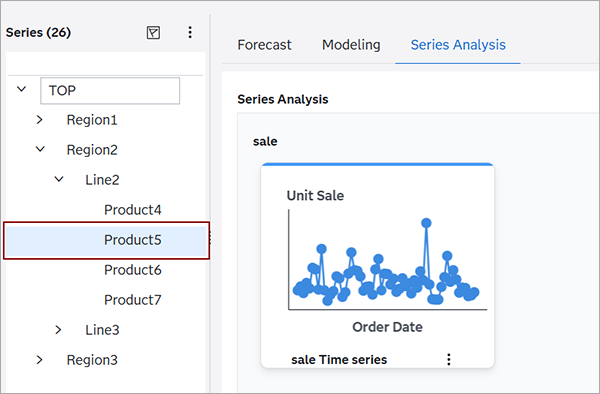
If Hierarchical Modeling is turned on, the Series pane shows the time series in a tree view.
Place an input variable in the canvas in the right pane.
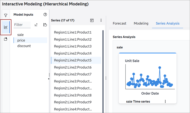
1. Select in the left pane.
  The dependent variable and independent variables for the project are displayed in the Model Inputs pane.
2. Select one or more of the input variables in the left pane and drag it to the canvas.
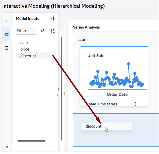
A row is added for each model input in the right pane. A time series plot is displayed by default.

As you add input variables to the canvas, each input is placed in a new row. You can drag and drop each row on the canvas to reorder them. You can also reorder the inputs by clicking in the top right corner of the canvas and selecting Reorder Analyses.

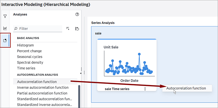
You can remove a row from the right pane by clicking in the top right corner of the row and selecting Remove. The initial row for the dependent variable cannot be removed.
Select an analysis to be displayed using one of these methods.
- Select in the left pane and drag an analysis to the row for the model input. You can select multiple analyses, but, for each input row, you can add only one type of each analysis
- Select an analysis from the drop-down menu in the row for the model input.
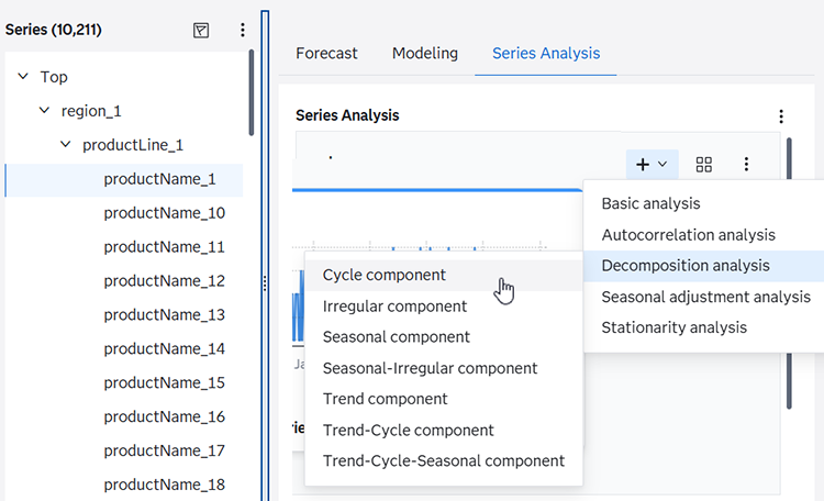
The plot for the selected analysis is generated and displayed in the tile.

At the bottom right corner of the input tile is a menu icon: . The menu provides these options.

Open

Displays a window with a larger view of the plot.

Settings

Use this option to change settings for certain settings, such as Lag or Decomposition method. Settings are not available for all of the analyses.

Log

If there is an error generating the plot, this option enables you to open and download the log to determine the cause of the error. The log option is not shown if the plot is generated successfully.

Remove

Removes the analysis from the model input row. The Time Series cannot be removed from the model input row.
Click and select Open. A larger plot is displayed in a new window.

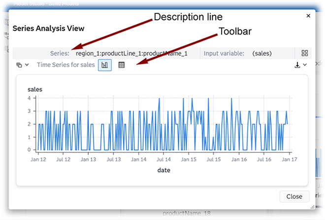
There is a description line at the top of the window showing the Series, which indicates the combination of BY variables for this time series. The line also shows the name of the Input variable and the icon, which adds all of the analyses in the row to the window.

Below the description line, there is a toolbar with these actions.
- ─ Displays a list of all of the analyses in this row. You can select another analysis to display it in this window.
- ─ Shows the plot for the analysis. This is the default. You can show the plot, the table, or both in this window.
- ─ Shows the table for the analysis. You can show the plot, the table, or both in this window.
- ─ Displays two options for downloading the data to your local drive. You can download Raw data or Formatted data.
- ─ Use this menu to open the Settings or the Log for the analysis. The Settings option is available only for analyses that have a Lag or Decomposition method that can be changed.
Click . You are prompted to save data for the table or graph that is displayed. If both are displayed, you are prompted to save data for both. The data is downloaded as a CSV file.
For Time Series, the data downloaded for the plot and table are the same.

For Histogram and Seasonal cycles, the plot data that is downloaded is different from the table. The data downloaded for the table provides the descriptive statistics for the time series. The data downloaded for the plot provides the values in the GTML that is used to create the plot.
Click at the top right corner of the model input row. This opens all of the analyses in the row in an enlarged window. This icon is also available when you open the enlarged view for a single analysis.
The view of multiple analyses provides this icon: . Clicking this icon opens the Display Settings window, which you can use to add more analyses to the window. This action also adds the analysis to the model input row.

Basic Analyses

The following basic analyses are available.

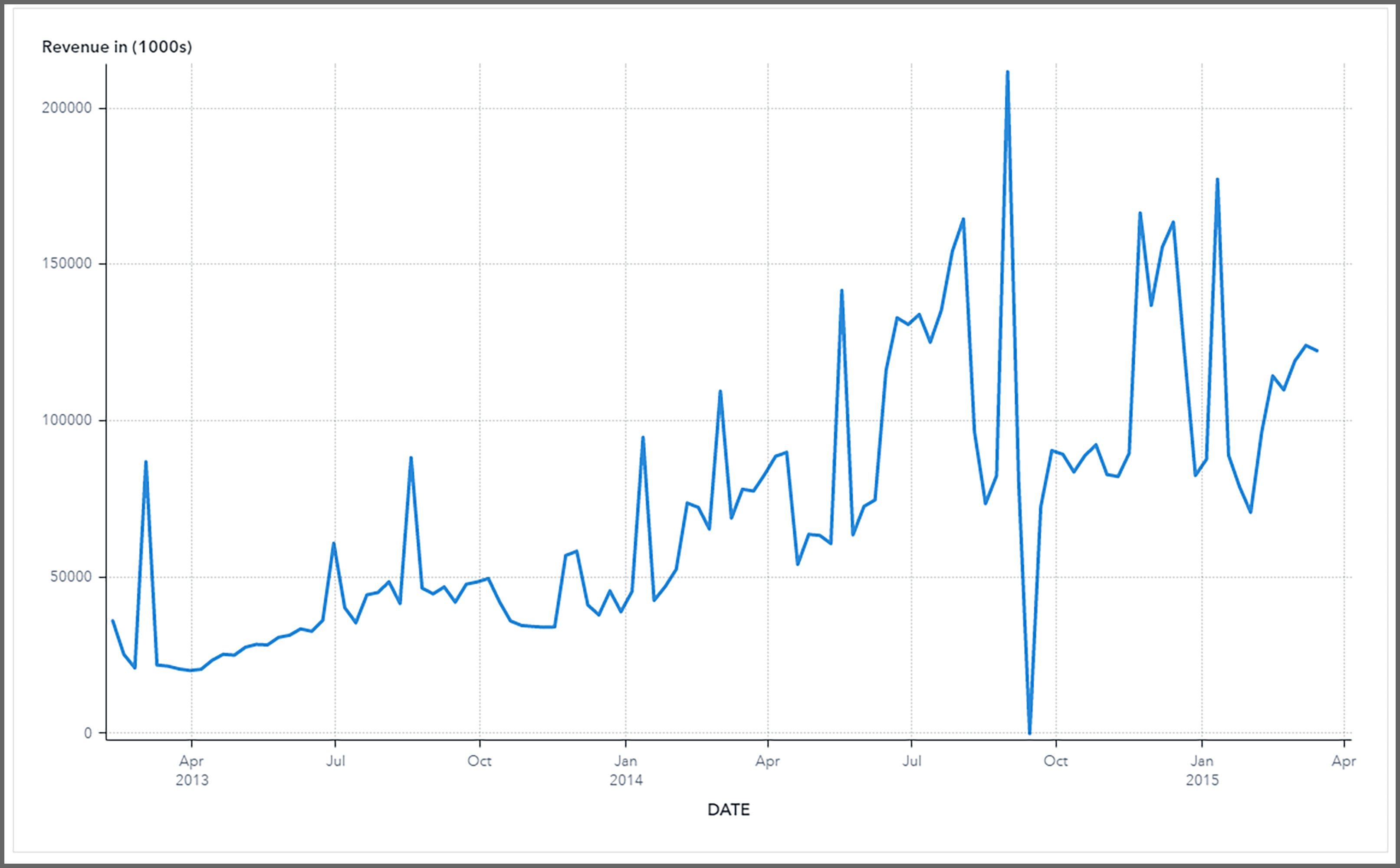
Time series Displays a plot of the selected time series over the historical time period
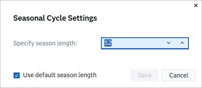
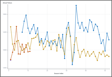
Seasonal cycles Displays any seasonal patterns for the selected time series at regular intervals in the plot You can change the seasonality (length of the season) for this plot to investigate different seasonal patterns. Using different seasonality specifications enables you to add multiple seasonal cycles to the canvas and compare the different plots. You cannot add a seasonal cycle to the canvas using the same season length as one that is already on the canvas. To change the seasonal cycle length, click and select Settings. The Seasonal Cycle Settings window is displayed. If you click View Details, you can also change the seasonal cycle length in the larger view of the plot using the menu icon in the upper right corner.
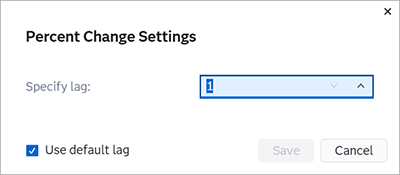
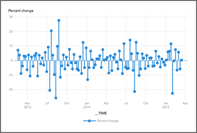
Percent change Displays the percent difference between each time period for the selected time series You can change the number of lags for which the change is shown in the time line. By default, each change shows the percent difference from the previous measurement (lag=1). For example, for monthly data (interval=month), for the default lag of 1, the first measurement on the plot starts at the second month and shows the percent difference from the prior month. However, if you change the lag to 3, then the first measurement on the plot starts at the fourth month and shows the percent difference from three months before. Changing the default lag specification enables you to add more percent change plots to the canvas for comparison. To change the lag specification, click and select Settings. The Percent Change Settings window is displayed. If you click View Details, you can also change the lag specification in the larger view of the plot using the menu icon in the upper right corner.
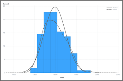
Histogram Displays a series of columns representing the frequency of the selected time series
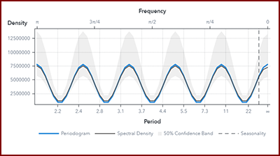
Spectral Density Shows the periodogram and the estimate of the spectral density of the selected time series.

Stationarity Analyses

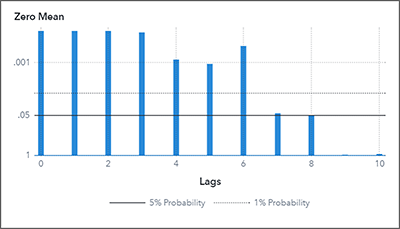
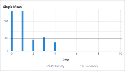
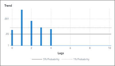
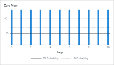
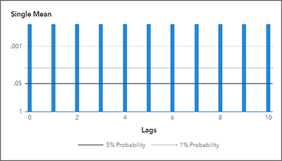
These plots are used to test zero-mean stationarity, single-mean stationarity, and linear-time trend stationarity. For zero-mean stationarity, a unit root test is conducted for an AR(p) model with zero mean for different values of lag p. For single-mean stationarity, a unit root test is conducted for an AR(p) model with a nonzero mean for different values of lag p. For trend stationarity, a unit root test is conducted for an AR(p) model with linear-time trend for different values of lag p.

If seasonality for the time series is d and 2<= d <= 12, then seasonal unit root tests are conducted for zero-mean and single-mean AR(p)(d) models for different values of lag p.

Note: Requesting a seasonal unit root test when seasonality is less than 2 or greater than 12 results in an error.

For more information, see Stationarity Tests and PROBDF Function for Dickey-Fuller Tests in the SAS/ETS User's Guide.

Each plot shows the logarithm of significance probabilities for unit root tests for different lag values p. The plots show log scale formats. The plot CSV file contains the raw values for the plot. There is a difference between the values in the plot CSV file and the values that are displayed when you hover over the plot. The following stationarity analyses are available.

Zero Mean Unit Root Test Probabilities (Log Scale) Test of unit root for the zero-mean model at different lags. In the table view, the Unit Root Test Code column shows `ZM` for zero mean stationarity.
Single Mean Unit Root Test Probabilities (Log Scale) Test of unit root for the nonzero mean model at different lags. In the table view, the Unit Root Test Code column shows `SM` for single mean stationarity.
Trend Unit Root Test Probabilities (Log Scale) Test of unit root for the trend model at different lags. In the table view, the Unit Root Test Code column shows `TR` for linear time trend stationarity.
Zero Mean Seasonal Unit Root Test Probabilities (Log Scale) Test of seasonal unit root for the zero-mean model at different lags. In the table view, the Unit Root Test Code column shows `ZM` for zero mean stationarity.
Single Mean Seasonal Unit Root Test Probabilities (Log Scale) Test of seasonal unit root for the nonzero-mean model at different lags. In the table view, the Unit Root Test Code column shows `SM` for single mean stationarity.

Autocorrelation Analyses

The following autocorrelation analyses are available.

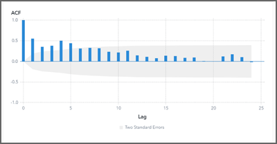
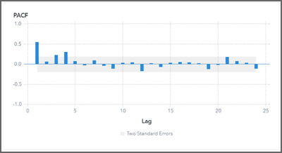
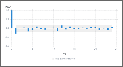
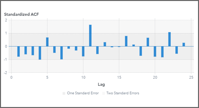
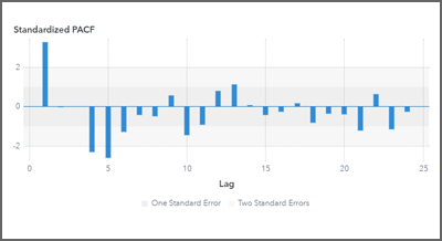
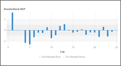
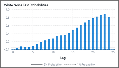
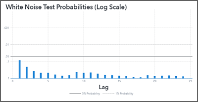
Autocorrelation Function Displays a plot of autocorrelation estimates. The number of lags shown can vary depending on the seasonality of the time series.
Partial Autocorrelation Function Displays a plot of partial autocorrelation estimates. The number of lags shown can vary depending on the seasonality of the time series.
Inverse Autocorrelation Function Displays a plot of inverse autocorrelation estimates. The number of lags shown can vary depending on the seasonality of the time series.
Standardized Autocorrelation Function Displays a plot of autocorrelation estimates on the normalized series. The number of lags shown can vary depending on the seasonality of the time series.
Standardized Partial Autocorrelation Function Displays a plot of partial autocorrelation estimates on the normalized series. The number of lags shown can vary depending on the seasonality of the time series.
Standardized Inverse Autocorrelation Function Displays a plot of inverse autocorrelation estimates on the normalized series. The number of lags shown can vary depending on the seasonality of the time series.
White noise probability test Displays the significance probabilities of the Ljung-Box chi-square statistic at various lag values of an input series. Probability values that are greater than the 1% probability threshold suggest a lack of autocorrelation in the preceding lags. Probability values that are greater than the 5% probability threshold suggest a strong lack of autocorrelation in the preceding lags. If the plot shows a strong autocorrelation at the most lags, it indicates that the series needs functional transformation or differencing for fitting a model. Strong autocorrelation at most lags indicates that the series is not stationary. Some common techniques for such series are to functionally transform or difference the series before fitting a model, or to fit a model with structural ability to account for the nonstationarity.
White noise probability test (log scale) Shows the significance probabilities of the Ljung-Box chi-square statistic at various lag values on a log scale. Probability values that are greater than the 1% probability threshold suggest a lack of autocorrelation in the preceding lags. Probability values that are greater than the 5% probability threshold suggest a strong lack of autocorrelation in the preceding lags. Strong autocorrelation at most lags indicates that the series needs functional transformation or differencing before fitting a model. Some common techniques for such series are to functionally transform or difference the series before fitting a model, or to fit a model with structural ability to account for the nonstationarity. This plot shows log scale formats. The plot CSV downloads the raw values for the same. There is a difference in the plot CSV values and the values seen on hovering the plot.

Decomposition Analyses

You can generate decomposition analyses for the model inputs. Classic decomposition breaks the time series into the following components.

Trend
Cycle
Seasonal
Seasonal-irregular
Trend-cycle
Trend-cycle-seasonal

Decomposition analysis is performed when the seasonality is greater than or equal to 2. If seasonality is less than 2, an error is generated.

The decomposition method determines the mode of the decomposition to be performed. There are four decomposition methods: additive, log-additive, pseudo-additive, and multiplicative. After you add a decomposition analysis to the canvas in Series Analysis, click Options on the analysis tile and select Settings. Select from one of the following methods.

Additive: specifies additive decomposition.
Log-additive: specifies log-additive decomposition. This method requires strictly positive time series. If this method is selected and the time series contains any nonpositive values, an error is generated.
Multiplicative: specifies multiplicative decomposition. This method requires strictly positive time series. If this method is selected and the time series contains any nonpositive values, an error is generated.
Pseudo-additive: specifies pseudo-additive decomposition. This method requires a nonnegative-valued time series. If the accumulated time series contains negative values, selecting the pseudo-additive method generates an error.
Automatic (default).: specifies multiplicative decomposition when the accumulated time series contains only positive values, pseudo-additive decomposition when the accumulated time series contains only nonnegative values, and additive decomposition under other circumstances. This method is selected by default.

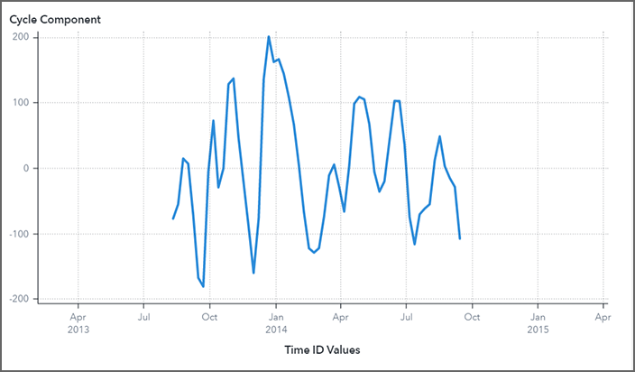
The following decomposition analyses are available.

Cycle component Displays the cycle component for the selected time series. The cycle component is obtained by subtracting the trend component from trend-cycle component. The Y axis shows a scaled-down measurement of the actual values.
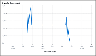
Irregular component Displays the irregular component for the selected time series. The irregular component is computed by using the seasonal-irregular component and the seasonal component. The Y axis shows a scaled-down representation of the actual values.
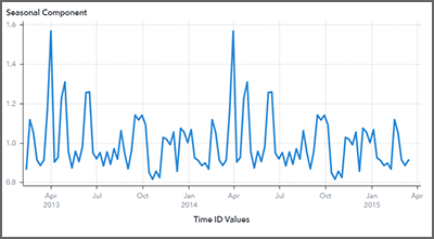
Seasonal component Displays the seasonal component for the selected time series. The seasonal component is obtained by averaging the seasonal-irregular component for each season. The Y axis shows a scaled down representation of the actual values.
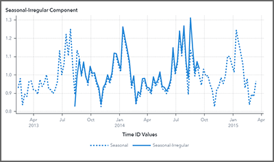
Seasonal-Irregular component Displays both the original series and the seasonal-irregular component for the selected time series. The seasonal-irregular component is computed by using the original series and the trend-cycle component. The Y axis shows a scaled-down representation of the actual values.
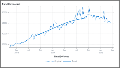
Trend component Displays both the original series and the trend component for the selected time series. The cycle component is obtained by subtracting the trend component from the trend-cycle component. The Y axis shows the actual values for the time series.
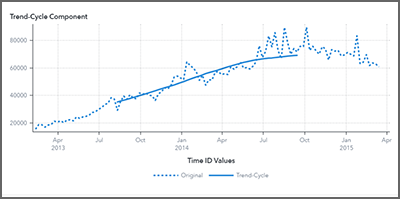
Trend-Cycle component Displays both the original series and the trend-cycle component for the selected time series. The trend-cycle component is computed from the centered moving average for the s-period. The Y axis shows the actual values for the time series.
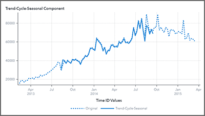
Trend-Cycle-Seasonal Component Displays both the original series and the trend-cycle-seasonal component for the selected time series. The trend-cycle-seasonal component is computed from the original series and the irregular component. The Y axis shows the actual values for the time series.

Seasonal Adjustment Analyses

You can generate seasonal adjustment analyses for the model inputs. The following seasonal adjustment analyses are available.

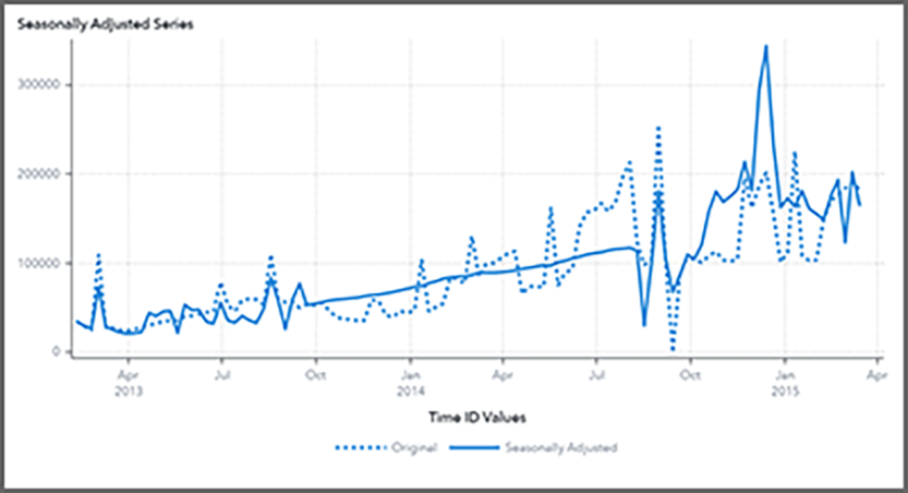
Seasonally adjusted series

Displays both the selected time series and its seasonally adjusted series. The seasonally adjusted series is computed from the trend-cycle component and the irregular component.

The Y axis shows the actual values for the time series.

Seasonally adjusted series

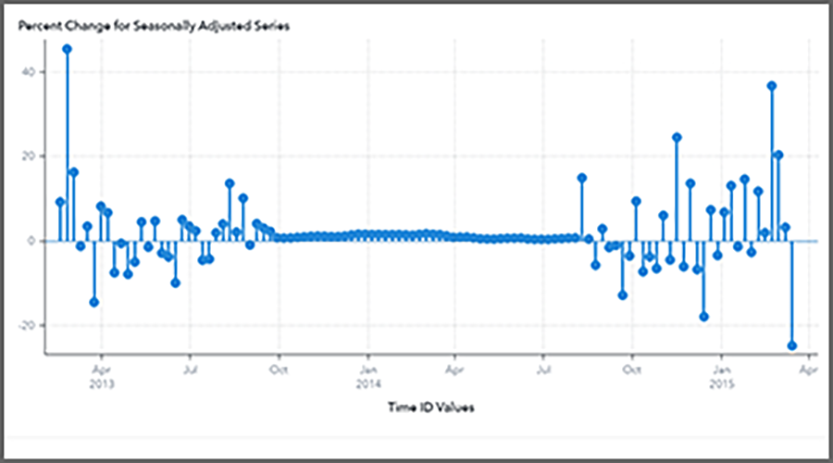
Percent change for seasonally adjusted series

Displays the percent difference between each time period for the seasonally adjusted series of the selected time series. The time period is set by the seasonality for the time interval and the lag. The default for lag is 1, but you can change it by clicking Options and selecting Settings.

See Seasonality to determine the seasonality based on the time interval set for the time variable.

Percent change for seasonally adjusted series

Seasonal Adjustment Formulas

Seasonal Adjustment Formulas
Component	Decomposition Method	Formula
original series	multiplicative
	additive
	log-additive
	pseudo-additive
trend-cycle component	multiplicative	centered moving average of O_t
	additive	centered moving average of O_t
	log-additive	centered moving average of
	pseudo-additive	centered moving average of O_t
seasonal-irregular component	multiplicative	$s , i sub t , equals , s sub t , i sub t , equals . fraction o sub t , over t , c sub t end fraction. Click image for alternative formats.$
	additive
	log-additive
	pseudo-additive	$s , i sub t , equals , s sub t , plus , i sub t , minus 1 equals . fraction o sub t , over t , c sub t end fraction. Click image for alternative formats.$
seasonal component	multiplicative	seasonal Averages of SI_t
	additive	seasonal Averages of SI_t
	log-additive	seasonal Averages of SI_t
	pseudo-additive	seasonal Averages of SI_t
irregular component	multiplicative	$i sub t , equals . fraction s , i sub t , over s sub t end fraction. Click image for alternative formats.$
	additive
	log-additive
	pseudo-additive
trend-cycle-seasonal component	multiplicative	$t c , s sub t end sub , equals t , c sub t . s sub t end sub , equals . fraction o sub t , over i sub t end fraction. Click image for alternative formats.$
	additive
	log-additive
	pseudo-additive
trend component	multiplicative
	additive
	log-additive
	pseudo-additive
cycle component	multiplicative
	additive
	log-additive
	pseudo-additive
seasonally adjusted series	multiplicative	$s , eh sub t , equals . fraction o sub t , over s sub t end fraction . equals t , c sub t , i sub t. Click image for alternative formats.$
	additive
	log-additive	$s , eh sub t , equals . fraction o sub t , over exp of open , s sub t , close end fraction . equals exp of open t , c sub t , plus , i sub t , close. Click image for alternative formats.$
	pseudo-additive

The trend-cycle component is computed from the centered moving average for the s-period as follows:

$t , c sub t , equals . cap sigma with k equals negative left bracket s slash 2 right bracket below and with left bracket s slash 2 right bracket above . fraction y sub t plus k end sub , over 2 end fraction. Click image for alternative formats.$

The seasonal component is obtained by averaging the seasonal-irregular component for each season where and .

$s sub k plus j s end sub . equals . cap sigma with t equals k mod s below . fraction s , i sub t , over fraction t , over s end fraction end fraction. Click image for alternative formats.$

The seasonal components are normalized to sum to one (multiplicative) or zero (additive).