Working with Individual Models for a Time Series

Modeling Tab

The Modeling tab in Interactive Modeling is similar to the Modeling tab in the Forecast Viewer, but with some substantial differences. For more information about the Modeling tab in Forecast Viewer, see Modeling Tab for Forecast Viewer.

The Modeling tab includes a model selection list table and a plot for the time seriesan aggregation of transactional data into specified time intervals and sorted according to unique combinations of the default attributes (BY variables) that is selected in the Series pane. By default, the first item in the list is selected in the Series pane. The contents in the model selection list are updated as you select other time series in the list. Select a model in the table by clicking on the row for the model. The row is highlighted and the plot below is updated based on the forecasts from that model. You can use the table to compare the different models before overriding the selected champion model.

Model Selection List Table

Each model in the table is categorized by one of the following types.

Predecessor

These models provide the forecasts from one of the preceding modeling nodes.

System-generated

These models are generated by Interactive Modeling. Generated models are the candidate models that would be generated by the equivalent of an Auto-forecasting node when it is run using the default selections. If you have an Auto-forecasting node preceding the Interactive Modeling node with the default selections, the generated forecasts and selection criteria should be the same.

If you right-click one of these models, you can select it as the new champion or create a copy of it with different settings.

Note: The usage of independent variables and eventsan incident that disrupts the normal flow of any process that generates the time series. Examples of events are holidays, retail promotions, and natural disasters. in system-generated ARIMA models are automatically set to Force to use if their inclusion does not cause the model to fail.

Custom

These models are created by users. Models can be created from scratch or can be copies of other models listed in the table. You can use the options in the Toolbar or right-click actions to create custom models. Models that are added to time series from the repository are also classified as custom models.

For more information, see Creating Models.

The table in the Modeling tab lists the predecessor modeling nodes and the system-generated models. If an Ensemble node is a predecessor, it is listed as follows:

• The Ensemble node indicates its champion predecessor model (for example: "Best of Seasonal Model") when a time series at the lowest level of the hierarchy is selected.
• If Hierarchical Modeling is turned on and a higher level in the hierarchy is selected in the Series pane, it simply indicates "Aggregated forecasts from Ensemble node".

Champion selection statistic

When Interactive Modeling is run, the models in the model selection list are assessed to determine the champion. System-generated models are not included in this assessment. By default, only the predecessor nodes are included in the assessment. If custom models have been added to any of the time series, they are included in the assessment only if Custom models has been checked under under Automatic Forecast Selection, in the right pane. If a model is manually selected as the champion, the other models in the list are not considered for champion.

The models in this table are sorted by the out-of-sample statistic of the Automatic Forecast Selection when an out-of-sample regionthe number of time periods before the end of the data that are removed when fitting models. After model selection, forecasts are generated in the out-of-sample region and then compared to the actual data to determine accuracy. is defined in project settings. If an out-of-sample region is not defined in project settings, the models are sorted by in-sample statistics of the Automatic Forecast Selection.

If an out-of-sample region is specified for this project, the out-of-sample statistics are shown for each of the models. The out-of-sample statistics are used to determine the champion predecessor node. The champion modeling node is indicated with this icon: .

MAPE is the default statistic to determine champion model for each predecessor node. You can change this selection criteria using the Model selection criterion setting in Model suggestions.

By default, the champion predecessor model is selected using RMSE. RMSE is the default under the Automatic Forecast Selection settings for Interactive Modeling. To use another statistic for selecting the champion, see Specify criterion.

Note: For hierarchical forecasting, the statistics of fit value shown for the predecessor model differs from the one shown in the Modeling tab of the Forecast Viewer. The measure shown in Interactive Modeling is the reconciled value from the OUTSTAT table. The measure in the Modeling tab for Forecast Viewer is the value before reconciliation from the OUTSELECT table.

The contents of the model selection list table depend on whether you select Inherit model selection list of predecessor modeling node in the options for Interactive Modeling.

Inherit the predecessor node's model selection list is turned off

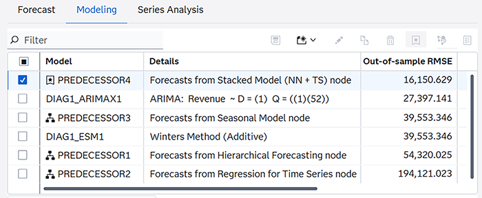
The predecessor modeling nodes are listed with the name PREDECESSOR, followed by a number if there is more than one preceding modeling node. For the selected time series, the predecessor node that has the best score for the selection criteria is marked as the champion (). In the figure below, the Details column shows the name of the predecessor modeling node. For example, PREDECESSOR3 is a Seasonal Model node. PREDECESSOR4 (Stacked Model) is marked as the champion because it has the best RMSE score.

• Model Selection List Table with Predecessor Nodes Listed

  

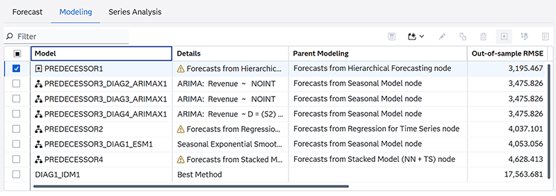
Inherit the predecessor node's model selection list is turned on

In this table, the model selection list includes the candidate models that are in the predecessor node's model selection list. In the figure below, there are four predecessor nodes. In this example, only PREDECESSOR3 (Seasonal Model) provides the candidate models from its model selection list. When the model selection list from a predecessor node is provided, the Details column does not display the name of the predecessor node. Instead, it displays information about each model provided by PREDECESSOR3. To determine the name of each predecessor, add the Parent Modeling column to the table. For information about adding, rearranging, and removing columns in a table, see Working with Tables in SAS Model Studio in SAS Visual Forecasting: Overview.

PREDECESSOR1 in this table is a Hierarchical Forecasting node, which does not provide a model selection list. For Hierarchical Forecasting, you can generate the Forecast Model Selection Graph table, but Interactive Modeling does not inherit it. For a list of modeling nodes that can provide their model selection list, see Inherit model selection list of predecessor modeling node.

• Model Selection List with Predecessor Models Listed

  

Right-click actions

The following right-click actions are available for all of the models in this table except for the predecessor model.

Compare selected models

After you select two or more models in the table, this option opens a window that displays all of the selection statistics for each selected model. The icon in the toolbar performs the same action.

Set as champion

This selects the model as champion. One of the predecessor models is initially set as champion. After you select a champion, you need to save the changes as described in Selecting a Different Champion Model.

Unselect champion

This changes the champion designation to the model that was originally designated as champion. After you deselect the champion model, you must save this change as described in Saving Your Changes in Interactive Modeling.

View status details

If a model generates a warning or error, use this option to get more information. You might need to download the logs for complete analysis.

Edit selected model

Opens the window to edit the model definition. This option is enabled only for custom models. This includes user generated ESM, ARIMA, and Subset (Factored) ARIMA models. You cannot edit system-generated or predecessor models or any model that is selected as the champion. If a custom model is included in a combination model, it cannot be edited.

The icon in the toolbar performs the same action.

Create a copy of the selected model

Opens a window where you can change the settings and save a new copy of the model. The icon in the toolbar performs the same action. This option is not enabled for predecessor models.

Note: Some models can provide a valid statistic of fita statistical value that is used to evaluate how well a forecasting model fits the historical series by comparing the actual data to the predicted values. in the In-sample MAPE column, even if the Details column shows a status code. Creating a copy of these models can result in a failed model. Try to make changes to the model specification to resolve the status error before you attempt to copy the model.

Delete selected model

Select one or more custom models for deletion. The icon in the toolbar performs the same action. You can delete only custom models. The following criteria must be true to delete a custom model.

• The model cannot be marked as champion.
• The model cannot be included in a combination model.

If multiple custom models are selected for deletion, only those models that meet these criteria are deleted.

Download

Select from these options:

• Download model specification code — Downloads the CASL code for the selected model and time series. See Downloading and Running Code for a Model for more information.
• Download model formatted data — Downloads the formatted data for the time series. This data differs from the seriesData.csv that is included in the Download all option. The data is formatted for your specific locale and there are two rows at the top that identify the model and the unique BY variable identification for the time series.
• Download all — Downloads the CASL code and time series data for this model. See Downloading and Running Code for a Model for more information.

Save to model repository

Saves the selected model to the model repository. See Saving Models to the Model Repository for more information.

Toolbar

The toolbar above the model selection list includes these icons. Some icons can also be selected using right-click actions. Those icons are explained in Right-click actions. The following icons do not have an associated right-click action.

Use this to create your own model. For more information, see Creating Models.

Opens the Model Details window that displays the properties of the selected model. This action is disabled for the predecessor node.

Plot for the Selected Time Series

A plot for the selected time series is displayed below the model selection list table. When you open the Modeling tab, it initially shows the Historical and forecast region plot for the selected model. These plots are based on the forecasts that correspond to the models generated by the Interactive Modeling node.

The toolbar over the plot includes these icons.

• — Downloads a CSV file with the data for the selected plot or table. You have a choice to download all tables and plots or only those that you select. You can choose to download the raw data or data formatted for your specific locale.
  Note: If you choose to download all tables and plots, in some cases they are not all downloaded. If you are missing any downloads, you can select the individual plot or table to download again.
• — Maximizes the plot or table to a separate window that can be resized
• — Displays all of the available plots and tables in one window. When you click this icon, all of the graphs and tables are opened in the tile view. From the tabs at the top of the tile view, you can select one of these plot and table groupings.
  • Forecast
  • Model fit
  • Basic error analysis
  • Error autocorrelation analysis

  Click Manage View Diagnostics to add or remove any plot or table from the tile view.

Use the View diagnostic plot/table menu to select among these other plots and tables.

Forecast

• Historical and forecast region — Shows the actual and fit or predicted values for the selected model and time series over the historical and forecasta numerical prediction of a future value for a specified time period for each unique combination of BY variable values horizonthe number of intervals into the future, beyond a base date, for which analyses and predictions are made. time periods.
• Forecast region only — Shows the predicted values for the selected model and time series over the forecast horizon time periods. If an out-of-sample region is specified for the project, it is included in the plot of the forecast region.
• Historical region only — Shows the actual and fit or predicted values for the selected model and time series over the historical time periods. If an out-of-sample region is specified for the project, it is not included in the plot of the historical region.
• Seasonal cycles — Displays any seasonal patterns for the selected time series at regular intervals in the plot.
• Model components — Shows the predicted values for a component of the selected model. For a description of each component, see Model Components.

Model fit

• Parameter estimates — Shows the values generated in the parameter estimation step. For a complete description of this table, see Parameter Estimates (OUTEST).
  Note: The parameter estimates table is not available for the predecessor node.
• Statistics of fit — Shows all of the calculated statistics of fit for the selected model and time series. The row with Region=FIT shows the statistics for the historical region. If an out-of-sample region is specified for the project, then the row with Region=FORECAST includes the statistics for the out-of-sample region.
• Unbiasedness test — The plot produced by this analysis shows the predicted values against the actual values and includes the estimates, standard errors, and significance-level indicators of the t test (asterisks next to the standard error) for intercept and slope parameters of the fitted regression line. An unbiased prediction would typically result in an insignificant intercept estimate (no asterisks) and a significant slope estimate (one or more asterisks). The slope estimates are indicated as follows:
  • ***: p-value <= 0.01
  • **: 0.01 < p-value <= 0.05
  • *: 0.05 < p-value <= 0.1
  • no asterisks: 0.1 < p-value

  The table produced by this analysis is an ANOVA table of a joint test of intercept=0, slope=1, from regressing the actual values on the predicted values. A large p-value for the F test indicates that predictions are unbiased.

Basic error analysis

• Prediction errors — Shows a plot over the historical region of the difference between the actual values and forecast values predicted by the model. Each error is calculated as the actual value minus the forecast value.
• Prediction error histogram — Shows the prediction errors in histogram format. The vertical bars represent the value-binned errors by percentage. The bell-shaped curve shows the normal distribution with mean and variance estimated from the prediction errors. The dotted line shows the kernel density estimate, which is a nonparametric estimate of the density function.
• Prediction error spectral density — Shows the periodogram and the estimate of the spectral density of the prediction errors.

Error autocorrelation analysis

• Autocorrelation function — Displays a plot of autocorrelation estimates. The number of lags shown can vary, depending on the seasonalitya regular change in time series data values that occurs at the same point in each time cycle. of the time series and the number of missing and nonmissing observations in the series.
• Standardized autocorrelation function — Displays a plot of autocorrelation estimates on the normalized error series. The number of lags shown can vary, depending on the seasonality of the time series and the number of missing and nonmissing observations in the series.
• Partial autocorrelation function — Displays a plot of partial autocorrelation estimates. The number of lags shown can vary, depending on the seasonality of the time series and the number of missing and nonmissing observations in the series.
• Standardized partial autocorrelation function — Displays a plot of partial autocorrelation estimates on the normalized error series. The number of lags shown can vary, depending on the seasonality of the time series and the number of missing and nonmissing observations in the series.
• Inverse autocorrelation function — Displays a plot of inverse autocorrelation estimates. The number of lags shown can vary, depending on the seasonality of the time series and the number of missing and nonmissing observations in the series.
• Standardized inverse autocorrelation function — Displays a plot of inverse autocorrelation estimates on the normalized error series. The number of lags shown can vary, depending on the seasonality of the time series and the number of missing and nonmissing observations in the series.
• White noise probability test — Shows the significance probabilities of the Ljung-Box chi-square statistic at various lag values. Probability values that are greater than the 1% probability threshold suggest a lack of autocorrelation in the preceding lags. Probability values that are greater than the 5% probability threshold suggest a lack of strong autocorrelation in the preceding lags.

  Lack of strong autocorrelation at most lags indicates that the residuals are white noise and model is a good fit. Probability values are valid and hence shown only for lag values that are greater than the number of parameters in the fitted model.

• White noise probability test (log scale) — Shows the significance probabilities of the Ljung-Box chi-square statistic at various lag values on a log scale. Probability values that are greater than the 1% probability threshold suggest a lack of autocorrelation in the preceding lags. Probability values that are greater than the 5% probability threshold suggest a lack of strong autocorrelation in the preceding lags.

  Lack of strong autocorrelation at most lags indicates that the residuals are white noise and model is a good fit. Probability values are valid and hence shown only for lag values that are greater than the number of parameters in the fitted model.

See Also

• Generating Output from SAS Model Studio in SAS Visual Forecasting: Overview
• Error Message When Selecting a Time Series from the Modeling Tab of Interactive Modeling

Using the Model Repository

The model repository stores models that have been created by users of SAS Visual Forecasting. The repository enables you to reuse these models for any time series in your project. The scope of the model repository is project wide. You cannot reuse models from one project in another project.

The model repository is populated with predefined models at project creation and when a project is imported. Custom models that you create in Interactive Modeling can be saved to the model repository, along with models created by other users for the same project. You can also save system-generated models to the model repository. You cannot save predecessor models or custom combination models to the model repository.

For a complete list of predefined models, see Predefined Models in the Model Repository.

Comparing Models

Follow these steps to compare models in the model selection list.

1. Select two or more models in the Compare column in the table.
2. Click in the toolbar above the table. You can also right-click in the table and select Compare selected models.

   This opens the Compare Statistics of Fit window. The time series plot shows the historical data and forecasts for each model that is selected. The table contains the calculated statistics of fit for each model.

   For each fit statistic, the best performing model is highlighted in yellow. The other models have lighter yellow backgrounds, according to their scores, and the worst performing model has no background color.

   If an out-of-sample region is specified for the project, you can select between the in-sample and out-of-sample statistics of fit above the table.

3. To add, remove, or arrange the fit statistics in the table, click at the top right of the table.

Selecting a Different Champion Model

The model selection list shows all of the predecessor models, system-generated models, and custom models available for the selected time series. The system-generated models are generated using Auto-forecasting with the default settings. The initial champion is selected from the predecessor models. You can select another model in this model selection list as the new champion for the selected time series.

You can select champion models for multiple time series. The changes do not go into effect until you save them. The models that are saved as champion replace the model that is currently selected as champion. When you are working with changes to champion models, any user working in the same Interactive Modeling node cannot see your changes until you save. For more information, see Saving Your Changes in Interactive Modeling.

Your selections for model champion can be lost if the pipeline is invalidated and you have to run the pipeline again. To preserve the selected model champions, go to the Pipelines tab, select the Interactive Modeling node, and select Reapply champion selection after the node is re-run in the right pane.

When the Interactive Modeling node is first run, the predecessor node that has the best score for the selection criteria is marked as the champion. To choose another model in this list as the champion, follow these steps.

1. Select the row for the model and click in the toolbar above the table. You can also right-click the row for the model and select Set as champion.

   The time series in the Series pane is updated with the icon. You can select other time series and set the champion model before you save the changes. Each time series is updated with this icon as you make changes.

   Note: The set champion icon, , is disabled for the currently selected champion. If you select another model as champion, you can right-click it and click Unselect champion it to return champion status to the initial champion.

   If you designate a system-generated model as champion, an exact copy of the model is created as a custom model and is designated as champion.

2. Save your changes before you exit Interactive Modeling. See Saving Your Changes in Interactive Modeling for more information.
3. The champion models that you chose for the selected time series replace the predecessor model that was originally selected. The Model Comparison and Output node need to be run again to complete the pipeline.

See Also

• Series Update Status

Saving Your Changes in Interactive Modeling

Actions such as selecting a different champion model. creating overrides, or setting the forecast values in the horizon are discarded if you exit Interactive Modeling without saving the change. Any work you do with overrides can be recovered if you lose your browser session with SAS Model Studio.

Follow these steps to save your changes.

1. When you are ready to save all of your changes, click the Save button above the table.

   The Save window is shown. All of the time series for which you have made changes are shown. Such changes include selecting a different champion model and setting the forecast values to zero or missing. You can deselect time series from the list.

   For any deselected time series, they remain in unsaved state unless you select the Discard changes for the series that are not selected.

   
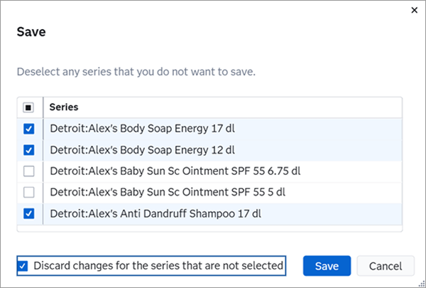
2. Click Save at the bottom of the window.

   Each time series with saved changes is shown in the Series pane with the icon.

   Note: If other users are working in the same Interactive Modeling node, they receive the following message after the change is saved.

   

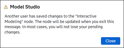
   After dismissing this message, the other users see the time series that were updated with the icon.

   If you deselect the champion status from a model, the initial predecessor becomes champion again, but this change must be saved.

3. To deselect a model that you have selected as champion, select the row with the champion model and click . The champion model for the selected time series reverts to the champion selected by the predecessor node.

   This icon acts as a toggle, turning the champion selection on and off. Each change with the champion icon requires the change to be saved.

Series Update Status

Some project updates can cause failures in models that are selected as champion in the Interactive Modeling node. If these failures occur, they are not noticed until Interactive Modeling is opened after another run of the pipeline. If there are failures, the Series Update Status window is shown when you open Interactive Modeling. This window lists all of the time series that have champion models that were saved but could not be applied after the project update.

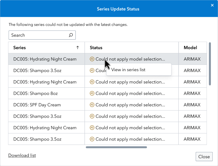
If there are many time series affected by the update, you can click Download list to download the complete list of time series to your local drive.

To address a failure, right-click the time series and select View in series list. The window closes and the selected time series is highlighted in the Series pane. Time series in with failures are indicated with the icon. You can also retrieve the Series Update Status window by clicking .

Here are some options to address the failed models.

1. For each failed model, take one of the following steps.
   • Select a different model as champion.
   • If it is a custom model, edit the model to correct the problem. Then reset the model as champion.
2. Save the changes as described in Saving Your Changes in Interactive Modeling.
3. Invalidate the Interactive Modeling node, as described in Invalidating a Single Node in a Pipeline.
4. Rerun the Interactive Modeling node.

After completing these steps, open the Interactive Modeling node again to verify that all of the failures have been fixed.

How Changes to the Hierarchy Affect Interactive Modeling

Changes to the hierarchy can affect the assignment of models in each time series in Interactive Modeling. Such changes include changing the hierarchy order, changing BY variable names, or changing the length of BY variables. You can expect the following changes in Interactive Modeling when the node is run again.

• Adding or removing BY variables results in the removal of custom models the next time the Interactive Modeling node is run.

  Changing the order of the project hierarchy can also remove custom models, but those models can be restored by changing the hierarchy back to its original order.

• Model specifications that are assigned to time series that no longer exist are deleted, with the exception of Hierarchical Modeling. In Hierarchical Modeling, the models are mapped to the series at a given level. If a custom model is added to a given level in the hierarchy, it persists even after BY variables are added or deleted unless that level no longer exists.
• Model specifications assigned to the BY variables with trailing spaces in the name are updated.
• Custom models that are no longer assigned to a time series are removed unless the hierarchy is simply reordered. After the hierarchy is reordered, custom models are still re-mapped to the lowest level of data in the hierarchy.
• Any changes to BY variables can result in failures to reapply custom changes that have been saved previously for one or more time series. Some examples of custom changes are setting of champion models or setting of forecasts in the horizon to zero or missing. Such failures are reported in the Series Update Status window with appropriate messages.