Modeling Nodes Provided by SAS Visual Forecasting

Hierarchy Levels

Hierarchy Levels

After the Data node is run, right-click this node and select Open to view the Hierarchy Levels table. The Name column shows the hierarchy levels along with the TOP level of the hierarchy. If a hierarchy is not defined, only Top is shown. Each row is a level in the hierarchy with its own nested pipeline that you can open, customize, and run.

After the node is run, reconciliation is performed. The success of the reconciliation is indicated above the table to the left. When reconciliation is running, you cannot open any of the nested pipelines in the table.

Sometimes the pre-reconciled predicted values can have missing values in the historical region due to lags used in modeling. During reconciliation, those missing values are filled with actual values. This adjustment causes a small difference between the weighted statistics of the pre-reconciled and reconciled forecasts at the reconciliation level.

The following controls are above the table to the right:

• Forecast Viewer — Opens the Forecast Viewer for the selected level. If a level is not selected, the Forecast Viewer for the lowest level in the hierarchy is opened.

The following icons perform actions that you can also select when you right-click a hierarchy level. If a level is not selected, these icons are disabled.

• — Runs the pipeline for the selected level.
• — Opens the pipeline for the selected level. You can also right-click the level and select Open.

  You can customize this nested pipeline like any other pipeline, with the exception that you cannot add a Hierarchical Forecasting, Hierarchical Forecasting (Pluggable), or another Hierarchical Modeling node to the nested pipeline.

• — Opens the list of pipeline templates for you to select a different pipeline.
• — If you change the pipeline for a level, this resets the pipeline back to the default.
• — Opens the following menu items.

  View reconciliation log

  Use this option if there is a failure in the hierarchy reconciliation.

Options

Default pipeline

Each pipeline is assigned using the Default pipeline setting for the Hierarchical Modeling node. If the value is changed after running the pipeline, it does not change the assigned pipeline for each level. To change the assigned pipeline to the new default setting, select one or more levels and click .

After successfully running the pipelines, if you reset the default pipeline, the modeling node and the following nodes show a status of Out-of-date. If you open the modeling node, the individual levels show a status of Completed. However, the nodes that are Out-of-date should be run again.

Reconciliation

Use the following settings to make changes to the reconciliation for this node.

Specify the reconciliation level

The reconciliation level is specified for this node by selecting a BY variable from the hierarchy. Consider the order of the default attributes (BY variables) defined on the Data tab. Select a variable to determine the type of reconciliation methodthe method that specifies the level in the hierarchy where the process of reconciliation starts. The following reconciliation methods are available: bottom-up method, middle-out method, and top-down method. .

• Select Top to perform top-down reconciliation.
• Select the variable at the bottom of the hierarchy to use bottom-up reconciliation. For example, if the hierarchy consists of two default variables, Location at the top and Name at the bottom, select Name to perform bottom-up reconciliation.
• You can select a variable in the middle level of the hierarchy to use middle-out reconciliation. For example, if the hierarchy consists of three default variables in the order of High, Medium, and Low (with High at the top), specify Medium to generate forecasts for that level and then reconcile forecasts for the upper and lower levels in the hierarchy.

By default, the reconciliation level set on the Data tab for the BY variables is used.

For a description of top-down, middle-out, and bottom-up reconciliation methods, see Understanding Hierarchy Reconciliation.

Disaggregation method during top-down disaggregation

specifies the type of disaggregation methoda method that specifies how the forecasts in the lower level of the hierarchy are reconciled when the reconciliation method is top-down or middle-out. The disaggregation method can reconcile the forecasts in either of the following ways: (1) by using the proportion that each lower-level forecast contributes to the higher-level forecast; or (2) by splitting equally the difference between the higher-level forecast and the lower-level forecasts. and type of loss function for top-down reconciliation. Select one of the following methods for top-down disaggregation:

• Difference — bases the loss function on the root mean square error (RMSE). This results in adjustments that are the (possibly weighted) mean difference of the aggregated child nodes and the parent node.
• Proportions — uses a loss function that results in reconciled forecasts that are the (possibly weighted) proportional disaggregation of the parent node.

Output Tables

Hierarchical Modeling automatically generates these tables. You can use the Save Data Node if you need to save any of these tables. You can add other models to the nested pipelines to generate other tables for any level in the hierarchy.

• Statistics of Fit (OUTSTAT)
• Descriptive Statistics (OUTSUM)
• User-Defined and Derived Attributes (MERGED_ATTRIBUTES)
• Forecasted Values (OUTFOR)

For Hierarchical Modeling, you can save the Statistics of Fit (OUTSTAT), Model Attributes (OUTMODELINFO), Forecasted Values (OUTFOR), , and Model Forecasts (OUTFOR_MODEL) tables for each level in the hierarchy.

Options

The following settings are available in the Options pane for the Naive Model node.

Naive model type

Select from the following.

• Moving average

  For this option, indicate the size of the moving average window.

• Random walk

  For this option, specify if you want the drift option.

• Seasonal random walk

  For this option, specify if you want the drift option.

Drift option for random walk models

If you choose a Random walk or Seasonal random walk model, you can add the drift option.

Window size for the moving average

Specify an integer, greater than 1, for the window size for the moving average model.

Output Tables

Naive Model automatically generates these tables. You can use the Save Data Node if you need to save any of these tables.

• Statistics of Fit (OUTSTAT)
• Descriptive Statistics (OUTSUM)
• User-Defined and Derived Attributes (MERGED_ATTRIBUTES)
• Model Attributes (OUTMODELINFO)
• Log Messages (OUTLOG)
• Forecasted Values (OUTFOR)

You can select the following optional tables. Select any tables that you want generated when this node is run. After the node is run, the tables can be saved using the Save Data Node.

• Parameter Estimates (OUTEST)
• Forecast Model Selection Graph (DIAGNOSEOUTFMSG)
• Model Forecast Components (OUTCOMPONENT)

Events and Handling for Missing Observations

The Naive Model does not support events.

For any time series with fewer than six nonmissing observations, an ESM model (ESM BEST) is used instead.

Overview

The Distributed Open Source Code node enables model developers, such as statisticians, data scientists, and forecasters, to provide their own open source code to perform time series forecasting for a project. When this node is added to a pipeline, it is not ready to run until the code has been added by the developer. SAS Visual Forecasting supports open source code written in R or Python.

The Distributed Open Source Code requires a deployment that contains a properly configured EXTLANG package. If the developer does not have the necessary access control permissions that are required by the EXTLANG package, the code does not work. For additional instructions, see External Languages Access Control Configuration. In addition, users who are running Distributed Open Source Node must be added to the CASHostAccountRequired custom group. For more information, see The CASHostAccountRequired Custom Group.

Once the environment is set up, the developer can follow these steps to add the code and run it.

1. In the Pipelines tab, add Distributed Open Source Code to the pipeline from the Nodes pane on the left.
2. With the node selected, in the right pane, select either R or Python for the code that you intend to use.
3. Click Open code editor. The code editor is opened.
4. Click to the left of the editor. This shows a list of variables to use in your code. See Variables Shared with the Open Source Code for a full description.

   The VF_PREDICT variable must be populated with the predictions from the open source code.

5. When you are ready to test your code, click to save your code, and then click Close.
6. Run the pipeline.

   When the node completes, check the following sources:

   • If the node fails, right-click the node and select Log to open the log and determine the source of the problem.
   • If the node is successful, right-click the node and select Results. On the Results page, click the Output Data tab and select the OUTOPENSRCSTATUS table. Check these status columns to determine whether the output of your open source code is working. If all status columns show all zeros, then the open source code is performing correctly. Otherwise, here are some steps to diagnose the cause of failure.
     1. If _ERRNO_ Status is not zero, review the OUTLOG table for more details.
     2. If Exit status code is not zero, refer to OUTOPENSRCLOG table to learn more about program errors.
     3. If the _MISSINGPREDICT_ column is not zero, review the open source program and make sure it generates forecast for all time periods in the forecast horizon region. The _MISSINGPREDICT_ column is labeled Specifies whether the forecasts are missing for all time periods in the forecast horizon on the Output Data tab.
     4. If _INVALIDPREDICT_ is not zero, review the open source program and make sure it generates a numeric array VF_PREDICT with length VF_LENGTH - VF_BACK. The _INVALIDPREDICT_ column is labeled Specifies whether the user program makes invalid modifications, such as deletion, reshaping, or garbling, to the VF_PREDICT variable on the Output Data tab.

After the code is included and has been run successfully, you can rename the node and save it to The Exchange for use in any other pipeline or project. You can add an Interactive Modeling node after it and compare the model comparison criteria with other models.

See Also

• Output Tables

Variables Shared with the Open Source Code

The Distributed Open Source Code internally constructs a program, referred to as the bridge program, which runs the timeData.runTimeCode action to execute various methods of the EXTLANG package. For more information, see the EXTLANG package documentation at External Languages Package. This bridge program interacts with the open source using shared variables.

After selecting the Distributed Open Source Code in a pipeline, click the Open button in the right pane to open the code editor. Then click to get a list of these variables.

The following variables are used by the open source code to return data to the bridge program for the Distributed Open Source Code node. The VF_PREDICT variable is required for the open source code. The program optionally can supply VF_ERROR, VF_LOWER, VF_UPPER, and VF_STD corresponding to the forecasts. If these arrays are valid, they appear in the OUTFOR table. Otherwise, the arrays are computed by the bridge program and a note is added to the OUTLOG table listing the array that is not feasible.

All of these arrays must be a length of VF_LENGTH - VF_BACK.

The following variables can be queried by the open source code to obtain information about the project and settings that can be used in generating the forecasts.

Best Practices for Open Source Code

• The code must provide predictions for the dependent variable. The predictions must be saved to the VF_PREDICT variable and matched to the time variable.
• The time ID variable passed to the open-source program is either SAS date value, SAS time value or SAS datetime value, depending on the data in the project. The user should be aware of their definitions. For more information, see Date, Time, and Datetime Constants in SAS Programmer’s Guide: Essentials.

  For Python code, you can use pandas.to_datetime function to convert SAS date value, SAS time value or SAS datetime value to pandas datetime. For example, the following code converts the SAS date value df.DATE to a proper argument that many Python modules are familiar with.

  df = pandas.DataFrame({'DATE': DATE, 'AIR': AIR}) 
  df.DATE = pandas.to_datetime(df.DATE, unit='D', origin=pandas.Timestamp('1960-01-01'))

  In this code, df is the pandas dataframe that contains time ID and another variable, AIR. The options unit= and origin= are defined according to the definition of SAS date value (the number of days from January 1st, 1960.)

• The length of the output forecast should match the size of historical region plus the size of horizon region.
• The output forecast should be an array. In Python, it can be a NumPy array or a simple list. It cannot be a pandas Series.

Examples

Example 1

The following shows example code of a seasonal random walk model for the Distributed Open Source Code node using the shared variables.

Python

for i in range(VF_SEASONALITY, VF_LENGTH):
    if i > VF_LENGTH - VF_LEAD:
        VF_PREDICT[i] = VF_Y[VF_LENGTH - VF_LEAD - VF_SEASONALITY]
    else:
        VF_PREDICT[i] = VF_Y[i - VF_SEASONALITY]

R

for (i in (VF_SEASONALITY+1):VF_LENGTH) {
    if (i > VF_LENGTH - VF_LEAD) {
        VF_PREDICT[i] <- VF_Y[VF_LENGTH - VF_LEAD - VF_SEASONALITY + 1]
    }
    else {
        VF_PREDICT[i] <- VF_Y[i - VF_SEASONALITY]
    }
}

The open source program can alternatively use VF_VARS[VF_YNAME] (in Python) or VF_VARS[[VF_YNAME]] (in R) in place of VF_Y. They all refer to the dependent variable array.

Example 2

If your deployment's CAS server has more than one CAS worker, you can use the following example to see how different time series get distributed among the multiple workers of the CAS server.

• 1. Open SAS Studio and use the following DATA step to start a CAS session and create a new data set. The new data set replicates the AIR data set 50 times to create 50 time series, each identified by the distinct value of the BYKEY variable.

     cas casauto;
     libname mycas cas;                                 
     options cassessopts=(caslib="Public");             
     
     data mycas.air50 (promote="yes");
        set sashelp.air;
        do bykey = 1 to 50;
           output;
        end;
     run;
     

  2. Open SAS Model Studio and create a Forecasting project using the new AIR50 data set. Make sure to select the variable BYKEY as a BY variable.
  3. Follow the steps in Overview to set up the pipeline and append the following Python code to any existing code that successfully generates forecasts.

     for i in range(VF_SEASONALITY, VF_LENGTH):
         if i > VF_LENGTH - VF_LEAD:
             VF_PREDICT[i] = VF_Y[VF_LENGTH - VF_LEAD - VF_SEASONALITY]
         else:
             VF_PREDICT[i] = VF_Y[i - VF_SEASONALITY]
     import socket
     print(socket.gethostname())

     You can add the last two lines of the preceding code to any Python code that successfully generates the forecasts. The print() statement writes to the OUTOPENSRCLOG table the name of the worker node where a particular time series is processed.

  4. Save the code and run the Distributed Open Source Code.
  5. When the node has finished running, right-click the node and select Results. The results page opens with the Summary tab showing.
  6. Select the Output Data tab.
  7. In the left pane under Logs, select OUTOPENSRCLOG.

     In the far right column, Text of the external language program log, you can find the name of the node that processes the series.

Output Tables

The following tables are automatically generated when running this modeling node. The tables can be saved to another caslib by using the Save Data Node.

• Forecasted Values (OUTFOR)
• Statistics of Fit (OUTSTAT)
• Model Attributes (OUTMODELINFO)
• User-Defined and Derived Attributes (MERGED_ATTRIBUTES)
• Log Messages (OUTLOG)
• Resource Usage Logs (OUTOPENSRCLOG)
• Model Status (OUTOPENSRCSTATUS)

Non-seasonal Model

The Non-seasonal Model node generates a list of appropriate non-seasonal model candidates for each time series, based on the model selection criteria that you choose. You can select between ESM, ARIMAX, and UCM models to be evaluated. After model selection, forecasts are generated for each time series using the selected model.

For ESM and UCM models, prebuilt options are available in PROC TSMODEL. For ARIMAX models, the search is performed over the models that have no seasonal AR, MA or differencing.

For a complete description of the settings that you can use, see Non-seasonal Model Settings.

This node is a pluggable model. You can edit the code to create your own modeling node. For more information, see Pluggable Modeling Nodes.

See Also

• Forecasting Process
• Generating Output from SAS Model Studio in SAS Visual Forecasting: Overview

Retired Series

This node is intended for time series that have been segmented based on patterns of inactivity as determined by the Demand Classification pipeline. It is not a good model for project data that has current active records. Retired Series does not support events.

This node does not generate forecasts. By default, all forecast values are set to missing. For information about changing this value, click for Retired Series in the Options pane.

This modeling node automatically generates these tables. You can use the Save Data Node if you need to save any of these tables.

• Statistics of Fit (OUTSTAT)
• Descriptive Statistics (OUTSUM)
• User-Defined and Derived Attributes (MERGED_ATTRIBUTES)
• Forecasted Values (OUTFOR)

You can also select the OUTFOR_HORIZON table. This table is optional. After the node is run, the OUTFOR_HORIZON table can be saved using the Save Data Node.

This node is a pluggable model. You can edit the code to create your own modeling node. For more information, see Pluggable Modeling Nodes.

See Also

• Generating Output from SAS Model Studio in SAS Visual Forecasting: Overview

Seasonal Model

This node generates a list of seasonal model candidates based on the model selection criteria that you select and generates forecasts. You can select between ESM, ARIMAX, and UCM as candidate models. ESM and ARIMAX are selected by default. The model selection is limited to seasonal models. For ESM and UCM models, prebuilt options are available in PROC TSMODEL. For ARIMAX, model selection is performed between models that have either seasonal AR, MA, or differencing greater than zero.

Time series that do not fit the seasonal model are forecast using the best ESM candidates. Candidate models include simple, linear, damped trend, additive seasonal, Winters multiplicative, and Winters additive models.

For a complete description of the settings that you can use, see Seasonal Model Settings.

This node is a pluggable model. You can edit the code to create your own modeling node. For more information, see Pluggable Modeling Nodes.

See Also

• Forecasting Process
• Generating Output from SAS Model Studio in SAS Visual Forecasting: Overview

Regression for Time Series

This node is intended to fit a pure regression model to the time series. This is accomplished by fitting an ARMA model with no intercept, no autoregressive (AR) component, and no moving average (MA) component. Omitting these components from an ARIMA model makes the model the equivalent of a regression model. For each time series, the node identifies the best regression model that can contain not only the independent variables and events that are available to use from the Data node, but also seasonal dummy variables and variables derived from the time index.

By default, the node creates seasonal dummy variables at the time interval of the input data or at a time interval that you specify. This option can be deselected. You can also select whether to include the observation index as an independent variable to capture linear effects, and to include the index squared and index cubed to capture higher order effects. If selected, these index-based features get included in the model only if they improve the model fit.

When this node is used in project data that has been segmented based on patterns determined by a Demand Classification pipeline, it is typically chosen as preferred modeling strategy for time series classified as INSEASON, which means activity occurs only during certain time periods. This model can also be a good fit for project data that consists of short time spans.

This node is a pluggable model. You can edit the code to create your own modeling node. For more information, see Pluggable Modeling Nodes.

For a complete description of the settings that you can use, see Regression for Time Series Settings.

See Also

• Forecasting Process
• Generating Output from SAS Model Studio in SAS Visual Forecasting: Overview

Temporal Aggregation Model

This node is intended for time series that are intermittent at the high-frequency level but seasonal at the accumulated low-frequency level. This modeling node forecasts high-frequency series using IDM and the low-frequency series are forecasted using one of the seasonal models that you select, such as ESM, ARIMA, or UCM. The results are then reconciled from the low-frequency level to the high-frequency level to yield the final forecasts.

The following table shows the time intervals used by this node. The project-level intervals on the left are specified on the time variable on the Data tab. These intervals are used to aggregate the high-frequency time series. As shown in the table, each high-frequency interval has a corresponding low-frequency interval, which is used to aggregate the low-frequency time series.

Any events used by this modeling node apply to the forecasts generated for the low-frequency interval.

Event support for this node was added in the 2025.01 release. Events are not supported for this node in projects imported from a deployment using a release prior to 2025.01. For projects imported from a prior release, you can add a new Temporal Aggregation Model to the pipeline and the new node supports events for the project. You need to make any modifications to the new node that you made to the previous Temporal Aggregation Model.

If the project is using a time interval that is not listed on the left, the low-frequency tables are not generated.

This node is a pluggable model. You can edit the code to create your own modeling node. For more information, see Pluggable Modeling Nodes.

For a complete description of the settings that you can use, see Temporal Aggregation Model Settings.

See Also

• Forecasting Process
• Generating Output from SAS Model Studio in SAS Visual Forecasting: Overview

Panel Series Neural Network

The Panel Series Neural Network modeling node provides forecasts by training a neural network based on user settings and develops a model to extract salient features across multiple time series. Neural networks consist of predictors (input variables), hidden layers, an output layer, and the connections between each of those items.

The Panel Series Neural Network modeling node is best suited for panels of time series with several interval independent variables. Independent variables for the neural network can be assigned in the Data tab or generated within the Feature Generation section of the node options. BY variables are automatically included as categorical inputs. This neural network cannot generate a model for the project without an independent variable.

For a description of the settings for this node, see Panel Series Neural Network Settings.

See Also

• Generating Output from SAS Model Studio in SAS Visual Forecasting: Overview
• Neural Network–Based Forecasting Strategies in SAS Viya

Multistage Model

The Multistage Model provides a general framework that combines time series models and feature extraction techniques to build a hierarchy-based forecasting system in two stages.

This modeling node is intended for a project with a defined hierarchy. If no BY variables are defined for the project, the forecast is generated using stage 1 time series model. For more information about hierarchies, see Defining the Hierarchy.

When working with the settings in the Options pane for Multistage Forecasting, consider any signals you might notice at different aggregationthe process of combining more than one time series to form a single series within the same time interval. For example, data can be combined into a total or an average. levels in the hierarchy. For example, in a retail scenario, time series signals such as trend or seasonalitya regular change in time series data values that occurs at the same point in each time cycle. might be best observed at a REGION or CATEGORY level. Setting this level as the stage 1 high level can better capture the time series signal using the stage 1 high-level time series forecast.

You might capture a stronger signal about how the sales respond to the price or promotionthe process of copying selected metadata and associated content within or between planned deployments of SAS software that could run different software releases. Methods of promotion include import and export processes, as well as explicit copies between two servers. This process is repeatable for a particular deployment. changes at the STORE or BRAND level. Setting this to the stage 1 low level allows the use of regression or neural network to model the price or promotion effect. At the lowest level, each STORE or SKU combination might have its own basic behavior that is not captured using the stage 1 models. These can be modeled separately in stage 2.

You can generate more a robust and reliable forecast by combining these elements:

• the time series signal that is modeled at the stage 1 high level
• the price or promotion effect that is modeled at the stage 1 low level
• the characteristics of each individual time series that is modeled at stage 2

This node is a pluggable model. You can edit the code to create your own modeling node. For more information, see Pluggable Modeling Nodes.

For more information about the individual settings for Multistage-forecasting, see Multistage Model Settings.

See Also

• Generating Output from SAS Model Studio in SAS Visual Forecasting: Overview

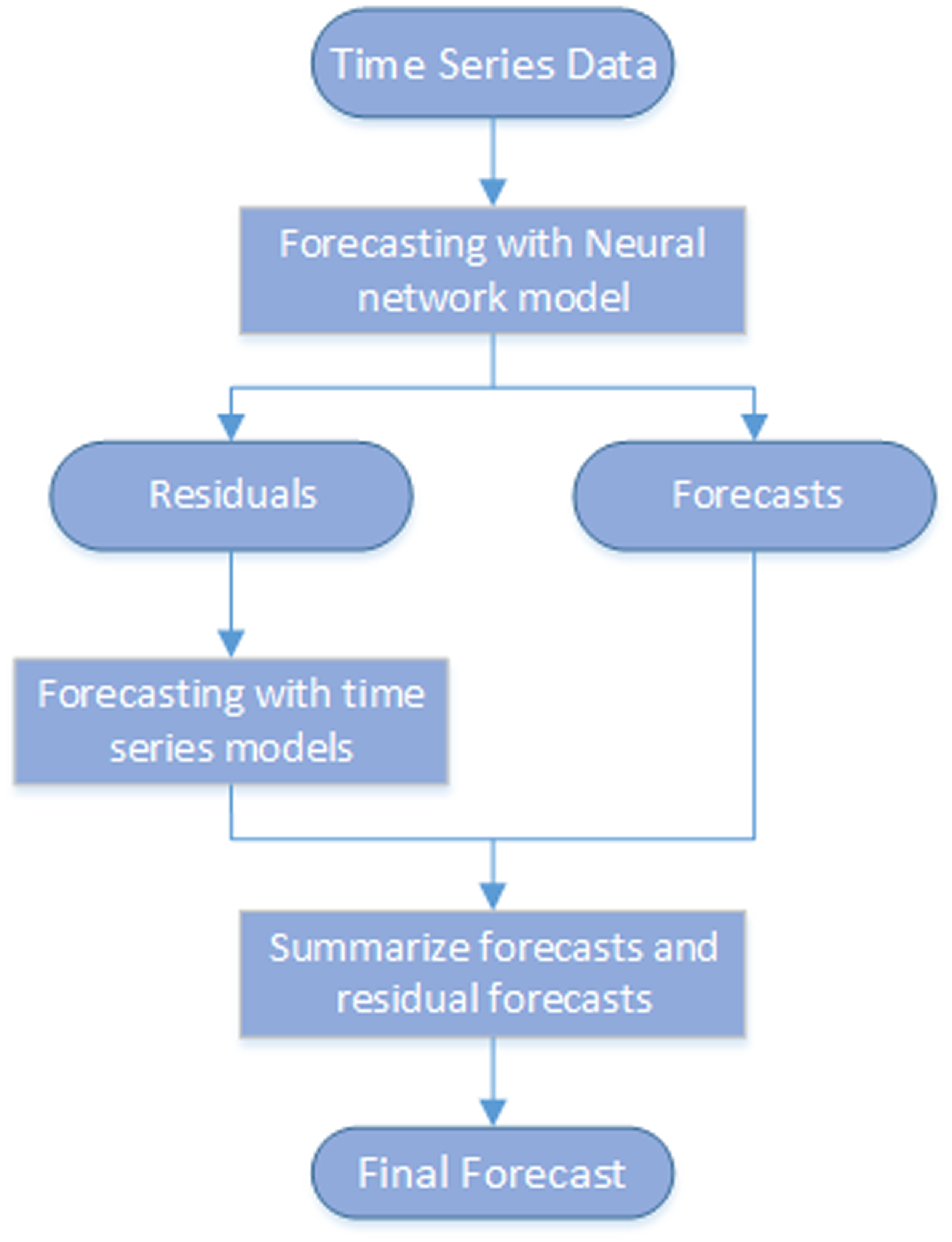
Stacked Model (NN + TS) Forecasting

See Also

• Generating Output from SAS Model Studio in SAS Visual Forecasting: Overview