VARMAX Procedure
Vector Autoregressive Fractionally Integrated Moving Average Model
Fractionally integrated models can be used to model stationary time series whose sample autocorrelation function decays slowly at large positive and negative lags. This behavior is often referred to as long-range dependence (LRD), long memory, or persistence; series that exhibit such behavior are called long-range dependent (LRD).
A typical parametric model for a k-dimensional series 
 whose individual components are LRD is the VARFIMA (vector autoregressive fractionally integrated moving average) model. It is obtained as a natural extension of the well-known class of ARFIMA models by fractionally integrating the individual components of a k-dimensional white noise series. For example, a bivariate VARFIMA
 series with no intercept term is given by

where B is the backshift operator;  is the identity operator;
  are the LRD parameters of the component series
  and
and  , respectively;
  ; and
; and  =
=  is a bivariate white noise series indexed by the set of integers
  with zero mean
  and covariance
  .
.
The multivariate VARFIMA model is defined analogously. The matrix  is in general nondiagonal, which enables the VARFIMA model to capture dependence between the individual series.
The following statements plot a simulated bivariate VARFIMA series with  ,
,  , and Gaussian errors with
  and
and  :
:
data VARFIMA0D0;
   time = _N_;
   input y1 y2;
datalines;
1.6380971 1.877144

   ... more lines ...

0.3482938 4.8601886
1.5320803 2.8687495
;
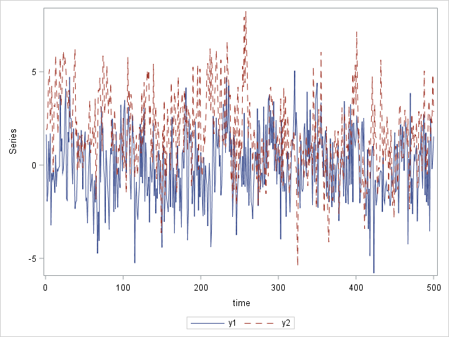
proc sgplot data = VARFIMA0D0;
   series x = time y=y1 / lineattrs=(pattern=solid);
   series x = time y=y2 / lineattrs=(pattern=dash);
   yaxis label="Series";
run;
Figure 19: Plot of the Data
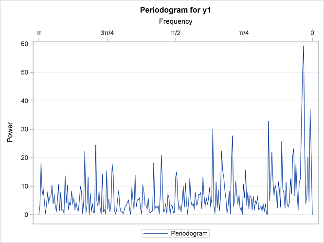
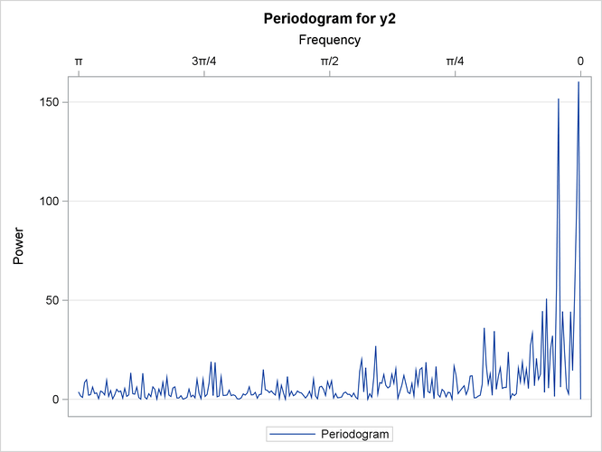
Before fitting a VARFIMA model to a data set, you should plot the series’ sample autocorrelation function to confirm its slow decay. It is also instructive to plot the periodogram of the series. In the presence of long memory, the periodogram explodes at frequencies near 0.
The following statements produce the periodogram and the sample autocorrelation function for the specified data:
ods graphics on;
proc timeseries data= VARFIMA0D0 plots = (periodogram acf);
   var y1 y2;
   spectra freq  / adjmean;
   corr / NLAG = 30;
run;
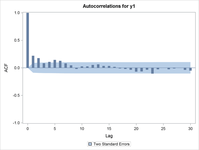
Figure 20: Sample Autocorrelation Functions of the Two Series
 |
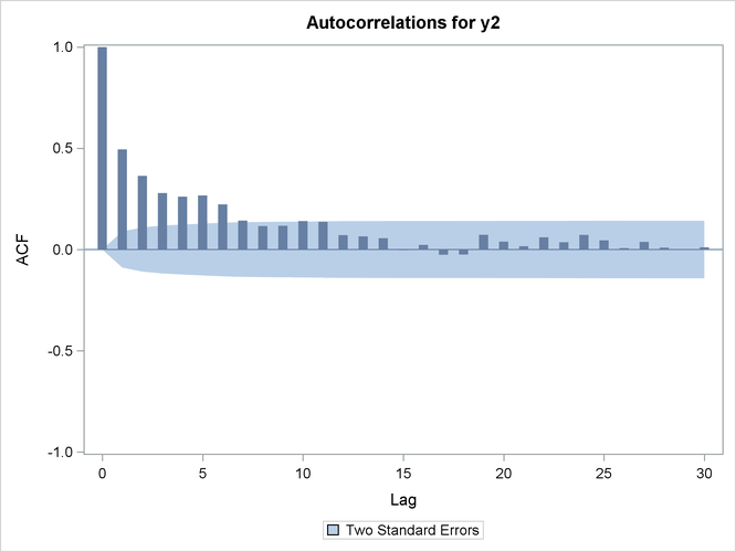 |
Figure 21: Periodograms of the Two Series
 |
 |
The magnitude of the LRD parameters  and
and  controls the memory of the two series. Series
  has a larger LRD parameter than series
  and hence is expected to exhibit longer memory. In the time domain, this effect is illustrated in Figure 20, where the autocorrelation function of series (right plot in Figure 20) decays more slowly than the autocorrelation function of series (left plot in Figure 20) with the increasing lag.
Figure 21 is the frequency domain analogue of Figure 20. In this case, the longer memory of series is reflected by its periodogram (right plot in Figure 21), which blows up higher than the periodogram of series (left plot in Figure 21) at frequencies near 0. Note the different scales used in the two plots.
The following statements fit the VARFIMA model with no intercept term to the data. The FI option in the MODEL statement specifies fractional integration.
proc varmax data = VARFIMA0D0;
   model y1 y2 / fi noint method = ML;
run;
Figure 22: Parameter Estimates for the VARFIMA Model
| Type of Model | VARFIMA(0,D,0) |
|---|---|
| Estimation Method | Maximum Likelihood Estimation |
| Model Parameter Estimates | ||||||
|---|---|---|---|---|---|---|
| Equation | Parameter | Estimate | Standard Error |
t Value | Pr > |t| | Variable |
| y1 | D1 | 0.20250 | 0.03555 | 5.70 | 0.0001 | |
| y2 | D2 | 0.38839 | 0.03053 | 12.72 | 0.0001 | |
| Covariances of Innovations | ||
|---|---|---|
| Variable | y1 | y2 |
| y1 | 3.20607 | 0.48068 |
| y2 | 0.48068 | 3.15651 |
The estimation method that PROC VARMAX uses by default for the VARFIMA series is maximum likelihood (for more information, see the section VARFIMA and VARFIMAX Modeling). All five parameter are estimated close to their true value and are significant.