VARMAX Procedure
VARFIMA and VARFIMAX Modeling
VAR and VARMA series are short-range dependent (SRD) in the sense that their autocovariance function dies out exponentially fast with the increasing lag. However, in many financial and macroeconomics applications, stationary yet persistent series arise, calling for models that have a slowly decaying autocovariance function and that are therefore more suitable to capture long-range dependence in the data.
The VARFIMA model captures both long-range and short-range dependence dynamics in a multivariate series. For a k-dimensional series  the VARFIMA
 model is defined as

where B and I are the backshift and identity operators; 
 , are the LRD parameters of the component series
  ,
,  ; and
; and  is a k-dimensional white noise series with zero mean
  and covariance
  .
.
The fractional integration operator  allows for long memory in the series. On the other hand,
  and
and  , which are the typical autoregressive and moving average matrix polynomials of orders p and q, respectively, capture the short-range dependence.
The VARFIMA series satisfies the multivariate long-range dependence definitions given in Kechagias and Pipiras (2015). Moreover, each component series , , satisfies the univariate time and frequency domain LRD definitions given in Beran et al. (2013). The following sections briefly review these definitions and show how you can detect long-range dependence in the data before fitting a VARFIMA model.
Autocorrelation and Spectral Density of VARFIMA Series
The diagonal components of the autocorrelation matrix function of a VARFIMA series satisfy the univariate LRD time domain definition

where  implies that
  and
and  . Similarly, the diagonal components of the spectral density matrix function of a VARFIMA series satisfy

for some  .
.
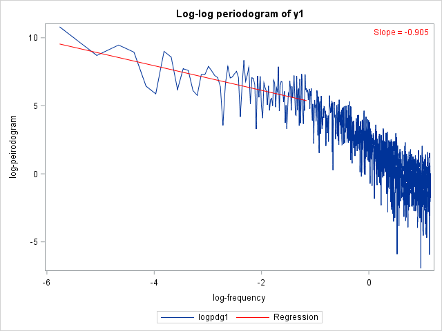
To obtain preliminary estimates of the LRD parameters, you can plot the logged periodogram values against the log of the Fourier frequencies  ,
,  and then fit a line for frequencies near 0. The slope of this line is expected to be equal to
  (the exponent in the right-hand side of the preceding relation). The following statements demonstrate this procedure for a synthetic VARFIMA
 series with
  2,000 and true parameters
  ,
,  ,
, 
 ,
,  ,
,  ,
,  ,
,  ,
,  ,
,  ,
,  , and
, and  :
:
data VARFIMA1D1;
   time = _N_;
   input y1 y2;
datalines;
1.495250048 2.694910375
4.503081454 1.42319642

   ... more lines ...

3.12049851 5.330308391
7.732287586 1.665071247
;
/* Compute the two periodograms */
proc spectra data = VARFIMA1D1 out = spectra;
   var y1 y2;
run;
/* Convert to log scale */
data logspectra;
   set spectra(firstobs=2);
   /* compute Fourier frequencies */
   j = _N_;
   pi = constant('pi');
   logfreq = log(2*pi*j/2000);

   logpdg1 = log(P_01);
   logpdg2 = log(P_02);

   /* Introduce weights where regression will be performed */
   wt = (1<= j <=100);
   keep wt logfreq logpdg1 logpdg2;
run;
/* Regression for log-periodogram of y1*/
proc autoreg data = logspectra(obs = 100);
   model logpdg1 = logfreq;
run;
/* Regression for log-periodogram of y1*/
proc autoreg data = logspectra(obs = 100);
         model logpdg2 = logfreq;
run;
The output from the two regressions is shown in Figure 86 and Figure 87.
Figure 86: Regression Estimates for y1
| Parameter Estimates | |||||
|---|---|---|---|---|---|
| Variable | DF | Estimate | Standard Error |
t Value | Approx Pr > |t| |
| Intercept | 1 | 4.3279 | 0.2885 | 15.00 | <.0001 |
| logfreq | 1 | -0.9051 | 0.1245 | -7.27 | <.0001 |
Figure 87: Regression Estimates for y2
| Parameter Estimates | |||||
|---|---|---|---|---|---|
| Variable | DF | Estimate | Standard Error |
t Value | Approx Pr > |t| |
| Intercept | 1 | 2.0811 | 0.3172 | 6.56 | <.0001 |
| logfreq | 1 | -0.5227 | 0.1369 | -3.82 | 0.0002 |
The following statements produce log-log plots of the two periodograms along with the regression lines:
/*Plot the periodograms in log-log scale*/
ods graphics on;

proc sgplot data = logspectra;
         series x = logfreq y = logpdg1 / lineattrs = (pattern = solid);
         reg y = logpdg1 x = logfreq / nomarkers weight = wt lineattrs =
                                       (thickness = 1 color = 'red' );
         inset "Slope = -0.905" / position = topright textattrs = (color = 'red');
         xaxis label = 'log-frequency';
         yaxis label = 'log-periodogram';
         title 'Log-periodogram of y1';
run;
proc sgplot data = logspectra;
         series x = logfreq y = logpdg2 / lineattrs = (pattern = solid);
         reg y = logpdg2 x = logfreq / nomarkers weight = wt lineattrs =
                                       (thickness = 1 color = 'red' );
         inset "Slope = -0.523" / position = topright textattrs = (color = 'red');
         xaxis label = 'log-frequency';
         yaxis label = 'log-periodogram';
         title 'Log-periodogram of y2';
run;
The final plots are shown in Figure 88.
Figure 88: Log-Log Periodogram Plots for the Two Series
 |
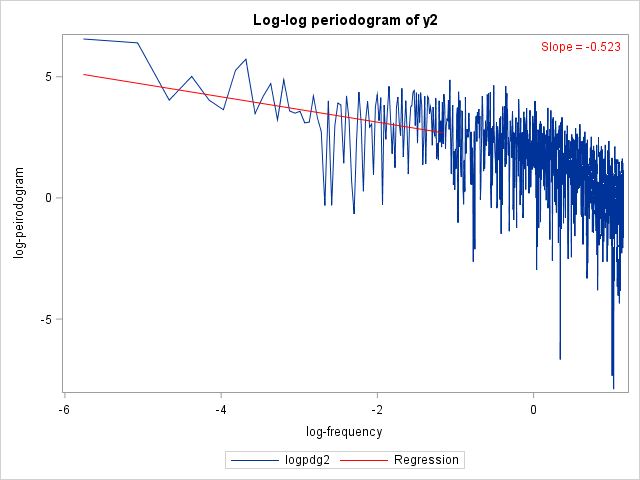 |
Dividing the slopes by 2 and removing the negative signs yields preliminary estimates for the LRD parameters,  and
and  .
.
Estimation
Estimation of all the parameters in the VARFIMA model is performed using the conditional likelihood Durbin-Levinson (CLDL) algorithm of Tsay (2010). This method uses the multivariate Durbin-Levinson algorithm, whose order of complexity is  , making it computationally feasible for small or medium sample sizes.
The initial values of the LRD parameters are obtained by the semiparametric estimator of Geweke and Porter-Hudak (1983). The initial values of the AR and MA parameters are obtained from least squares estimation on the fractionally differenced series  . The LRD parameters are restricted in the range
  . If an initial LRD parameter estimate is outside this range, then the chosen starting value is either
  or
or  for negative or positive initial semiparametric estimates, respectively.
Forecasting
One-step-ahead and multi-step-ahead forecasts for the VARFIMA series are based on a finite past. However, the h-step-ahead forecast errors for  are based on the infinite past except for VARFIMA series that have only MA components. In the latter case, the forecast errors are also based on a finite past.
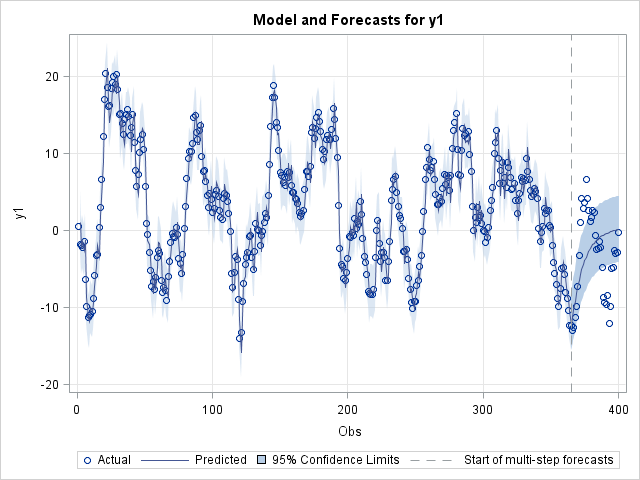
The following statements plot the h-step-ahead forecasts,  , for a bivariate synthetic VARFIMA series with
  and true parameters , , , , , , , , , , and . The statements also specify initial values for
  and
and  close to the true parameter values.
data VARFIMA1D1N4;
   time = _N_;
   input y1 y2;
datalines;
0.55596529 2.114409393
-1.842925215 3.415027987

   ... more lines ...

-2.86707489 1.147627529
-0.195787414 0.820107072
;
proc varmax data = VARFIMA1D1N4 plots = (forecasts);
         model y1 y2 / noint fi p=1 q=1;
         initial d(1) = 0.45, d(2) = 0.25;
         output out = forec back = 36 lead = 36;
run;
Figure 89: Plot of the Two Series and h-Step-Ahead Forecasts,
 |
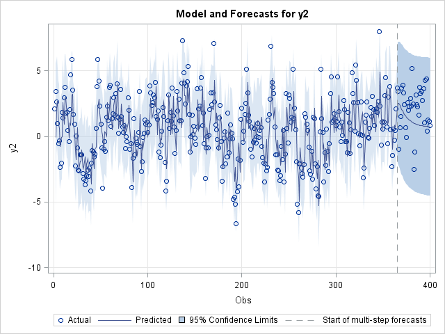 |
The BACK option in the preceding SAS statements is used to specify the point where the historical data ends and multi-step-ahead forecasting begins. Note that the BACK option does not affect estimation. The latter is performed using the whole data set, even when you specify the BACK option.
Impulse Response Functions
The impulse response functions of the VARFIMA series are calculated using the methodology of Chung (2001). The following statements produce the first 12 simple, accumulated and orthogonal impulse response functions and their corresponding standard errors for the VARFIMA series of the preceding example.
proc varmax data = VARFIMA1D1N4 plots = (impulse);
         model y1 y2 / noint fi p=1 q=1 print = (impulse = (all));
run;
VARFIMAX Modeling
The VARFIMAX series is defined as

where  ,
,  is an r-dimensional time series vector of exogenous variables and
  is the order s matrix polynomial defined as
  for some
  real matrices
  ,
,  .
.
The following statements estimate a bivariate VARFIMAX model:
model y1 y2 = x1 / fi p=1 q=1;