SEVERITY Procedure
Example 28.4 Estimating Parameters Using the Cramér–von Mises Estimator
(View the complete code for this example.)
PROC SEVERITY enables you to estimate model parameters by minimizing your own objective function. This example illustrates how you can use PROC SEVERITY to implement the Cramér–von Mises estimator. Let  denote the estimate of CDF at
  for a distribution with parameters
  , and let
  denote the empirical estimate of CDF (EDF) at that is computed from a sample
  ,
,  . Then, the Cramér–von Mises estimator of the parameters is defined as

This estimator belongs to the class of minimum distance estimators. It attempts to estimate the parameters such that the squared distance between the CDF and EDF estimates is minimized.
The following PROC SEVERITY step uses the Cramér–von Mises estimator to fit four candidate distribution models, including the LOGNGPD mixed-tail distribution model that was defined in Defining a Model for Mixed-Tail Distributions. The input sample is the same as is used in that example.
/*--- Set the search path for functions defined with PROC FCMP ---*/
options cmplib=(work.sevexmpl);

/*-------- Fit LOGNGPD model with PROC SEVERITY by using -------
  -------- the Cramer-von Mises minimum distance estimator -------*/
proc severity data=testmixdist obj=cvmobj print=all outest=est
     plots(histogram)=(pp conditionalpdf(rightq=0.8));
   loss y;
   dist logngpd burr logn gpd;

   * Cramer-von Mises estimator (minimizes the distance *
   * between parametric and nonparametric estimates)    *;
   cvmobj = _cdf_(y);
   cvmobj = (cvmobj -_edf_(y))**2;
run;
The OBJ= option in the PROC SEVERITY statement specifies that the objective function cvmobj should be minimized. The programming statements compute the contribution of each observation in the input data set to the objective function cvmobj. The use of the keyword functions _CDF_ and _EDF_ makes the program applicable to all the distributions. In addition to requesting the P-P plot, the PLOTS= option requests the conditional PDF plots of the body and tail regions. The CONDITIONALPDF option with the RIGHTQ=0.8 suboption specifies that the comparative conditional PDF plot be prepared for two regions:
the body region for loss values that are less than or equal to the 80th percentile
the right-tail region for loss values that are greater than the 80th percentile
Some of the key results prepared by PROC SEVERITY are shown in Output 28.4.1. The "Model Selection" table indicates that all models converged. When you specify a custom objective function, the default selection criterion is the value of the custom objective function. The "All Fit Statistics" table indicates that LOGNGPD is the best distribution according to all the statistics of fit. Comparing the fit statistics of Output 28.4.1 with those of Output 28.3.1 indicates that the use of the Cramér–von Mises estimator has resulted in smaller values for all the EDF-based statistics of fit for all the models, which is expected from a minimum distance estimator.
Output 28.4.1: Summary of Cramér–von Mises Estimation
| Input Data Set | |
|---|---|
| Name | WORK.TESTMIXDIST |
| Label | Lognormal Body-GPD Tail Sample |
| Model Selection | |||
|---|---|---|---|
| Distribution | Converged | cvmobj | Selected |
| logngpd | Yes | 0.12846 | Yes |
| Burr | Yes | 0.22681 | No |
| Logn | Yes | 0.16928 | No |
| Gpd | Yes | 35.98574 | No |
| All Fit Statistics | ||||||||||||||||
|---|---|---|---|---|---|---|---|---|---|---|---|---|---|---|---|---|
| Distribution | cvmobj | -2 Log Likelihood |
AIC | AICC | BIC | KS | AD | CvM | ||||||||
| logngpd | 0.12846 | * | 3657 | * | 3667 | * | 3667 | * | 3691 | * | 0.86572 | * | 1.04025 | * | 0.12957 | * |
| Burr | 0.22681 | 3724 | 3730 | 3730 | 3744 | 1.01660 | 2.27060 | 0.22826 | ||||||||
| Logn | 0.16928 | 3908 | 3912 | 3912 | 3922 | 0.92926 | 2.01192 | 0.16956 | ||||||||
| Gpd | 35.98574 | 5401 | 5405 | 5405 | 5415 | 9.85292 | 188.93299 | 35.99968 | ||||||||
| Note: The asterisk (*) marks the best model according to each column's criterion. | ||||||||||||||||
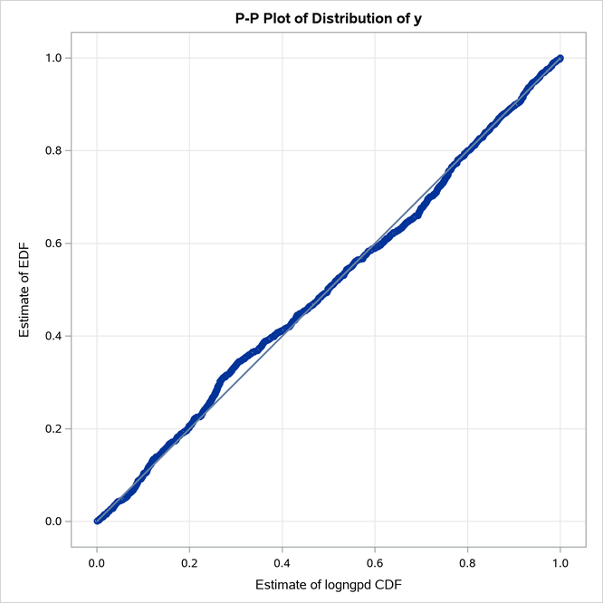
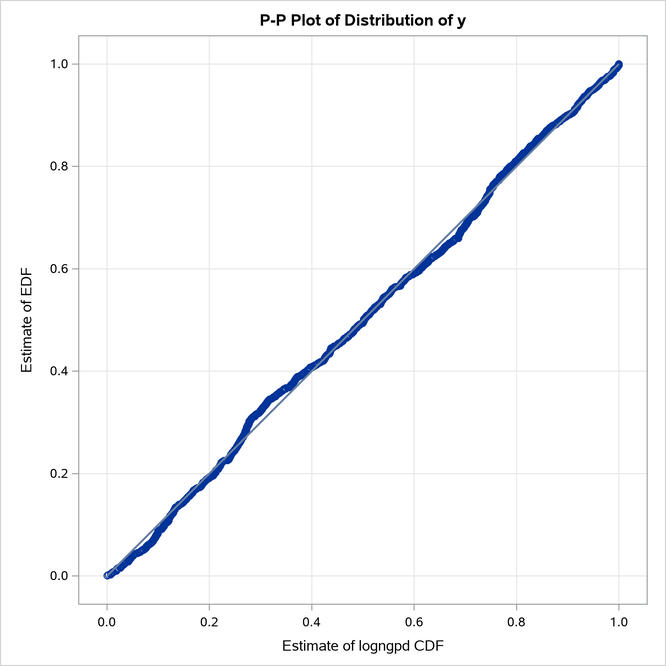
The P-P plots in Figure 22 provide a visual confirmation that the CDF estimates match the EDF estimates more closely when compared to the estimates that are obtained with the maximum likelihood estimator.
Figure 22: P-P Plots for LOGNGPD Model with Maximum Likelihood (Left) and Cramér–von Mises (Right) Estimators
 |
 |
The comparative conditional PDF plot in Figure 23 shows how the scaled density functions of different distributions compare in the body and right-tail regions. The scaling factor of each region reflects the probability that a loss value falls in that region. For the RIGHTQ=0.8 option, in the body region, the PDF values are scaled by a factor of 1.25 ( ), and in the right-tail region, the PDF values are scaled by a factor of 5 (
 ). Scaling makes the PDF plot in each region a true density function plot.
Figure 23: Comparison of the Conditional PDF Estimates of the Fitted Models
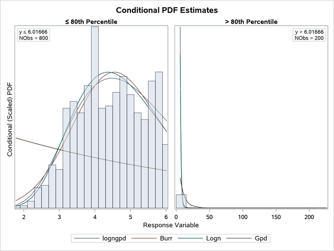
The right-tail plot in Figure 23 shows that the tail is heavy, but it is difficult to see the differences in the distributions because of the wide range of values in the tail. You can zoom in on specific portions of the tail by specifying the appropriate LEFTQ=, RIGHTQ=, and SHOWREGION= options. The following PROC SEVERITY step illustrates this:
proc severity data=testmixdist obj=cvmobj print=all inest=est
     plots=(conditionalpdf(leftq=0.75 rightq=0.975)
            conditionalpdfperdist(quantilebounds leftq=0.75 rightq=0.99
                                  showregion=(center right)));
   loss y;
   dist logngpd burr logn gpd;

   * Cramer-von Mises estimator (minimizes the distance *
   * between parametric and nonparametric estimates)    *;
   cvmobj = _cdf_(y);
   cvmobj = (cvmobj -_edf_(y))**2;
run;
The CONDITIONALPDF option specifies that the comparative conditional PDF plots be prepared for three regions: Y  75th percentile, 75th percentile
Y 97.5th percentile, and Y  97.5th percentile.
The suboptions of the CONDITIONALPDFPERDIST option specify that conditional PDF plots of individual distributions be prepared as follows:
The QUANTILEBOUNDS option specifies that the region boundaries be computed by using the quantile function of each distribution instead of the default of using percentiles. If you do not specify the QUANTILEBOUNDS option, then by default, PROC SEVERITY computes the region boundaries by using percentiles, which are empirical estimates of the quantile function.
The LEFTQ= and RIGHTQ= options specify that the plots be prepared for three regions:
Y Quantile(0.75), Quantile(0.75) Y Quantile(0.99), and Y Quantile(0.99). Note that the estimated quantile function might produce different values for different distributions, so the regions start and end at different values for different distributions. The SHOWREGION= option specifies that only the center and right-tail regions be plotted. The region between the LEFTQ= and RIGHTQ= values defines the center region. So in this example, the SHOW=CENTER option specifies that the region between Quantile(0.75) and Quantile(0.99) be shown. The SHOW=RIGHT option specifies that the right-tail region of values greater than Quantile(0.99) be shown. The example does not use the SHOW=LEFT option, so the left-tail region of values less than or equal to Quantile(0.75) is not shown.
The Work.Est data set is created by specifying the OUTEST= option in the first PROC SEVERITY step of this example. The use of that data set as the INEST= data set helps speed up the parameter initialization and estimation process significantly and enables you to explore different plotting options quickly.
The comparative conditional PDF plot that is prepared by the preceding PROC SEVERITY step is shown in Figure 24. It clearly shows the difference between different distributions in the three regions.
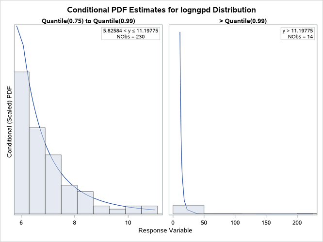
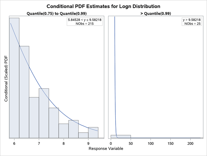
The "All Fit Statistics" table in Output 28.4.1 indicates that lognormal distribution is the best contender to the LOGNGPD distribution according to the EDF-based statistics of fit. The individual conditional PDF plots of the LOGNGPD and lognormal models are shown in Figure 25. Comparing the two plots shows that the LOGNGPD distribution has a better fit than the lognormal distribution in the right-tail region. The information in the insets of each plot indicates that although the Quantile(0.75) values of both distributions are closer to each other, the Quantile(0.99) values are significantly different. The larger Quantile(0.99) value of the LOGNGPD distribution confirms that it has a heavier tail than the lognormal distribution.
Figure 24: Comparative Conditional PDF Plots with Zoomed-In Tail Portions
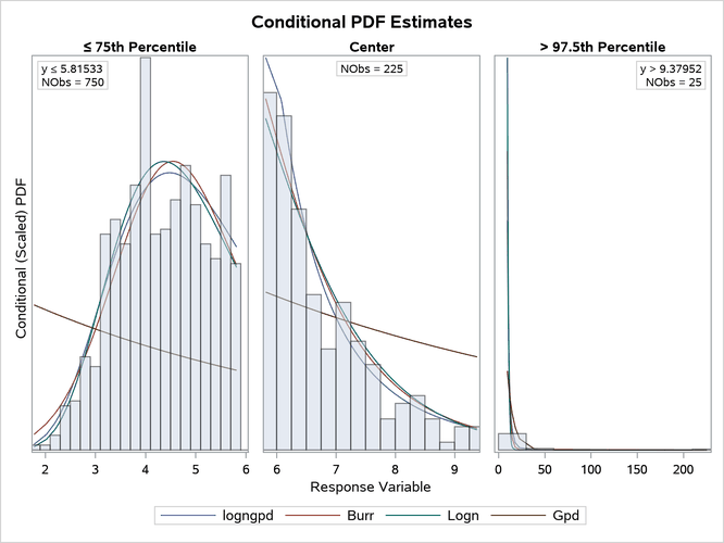
Figure 25: Conditional PDF Plots for Right-Tail Regions of LOGNGPD (Left) and Lognormal (Right) Models
 |
 |