SEVERITY Procedure
Example 28.3 Defining a Model for Mixed-Tail Distributions
(View the complete code for this example.)
In some applications, a few severity values tend to be extreme as compared to the typical values. The extreme values represent the worst case scenarios and cannot be discarded as outliers. Instead, their distribution must be modeled to prepare for their occurrences. In such cases, it is often useful to fit one distribution to the non-extreme values and another distribution to the extreme values. The mixed-tail distribution mixes two distributions: one for the body region, which contains the non-extreme values, and another for the tail region, which contains the extreme values. The tail distribution is usually a generalized Pareto distribution (GPD), because it is good for modeling the conditional excess severity above a threshold. The body distribution can be any distribution. The following definitions are used in describing a generic formulation of a mixed-tail distribution:

PDF of the body distribution

CDF of the body distribution

PDF of the tail distribution

CDF of the tail distribution

scale parameter for the body distribution

set of nonscale parameters for the body distribution

shape parameter for the GPD tail distribution

normalized value of the response variable at which the tail starts

mixing probability
Given these notations, the PDF  and the CDF
  of the mixed-tail distribution are defined as


where  is the value of the response variable at which the tail starts.
These definitions indicate the following:
The body distribution is conditional on
 , where X denotes the random response variable.
 The tail distribution is the generalized Pareto distribution of the
 values.
 The probability that a response variable value belongs to the body is
. Consequently the probability that the value belongs to the tail is  .
.
The parameters of this distribution are , , , , and . The scale of the GPD tail distribution  is computed as

The parameter is usually initialized using a tail index estimation algorithm. One such algorithm is Hill’s algorithm (Danielsson et al. 2001), which is implemented by the predefined utility function SVRTUTIL_HILLCUTOFF available to you in the Sashelp.Svrtdist library. The algorithm and the utility function are described in detail in the section Predefined Utility Functions. The function computes an estimate of  , which can be used to compute an initial estimate of as
  , where
  is the estimate of the scale parameter of the body distribution.
The parameter is usually determined by the domain expert based on the fraction of losses that are expected to belong to the tail.
The following SAS statements define the LOGNGPD distribution model for a mixed-tail distribution with the lognormal distribution as the body distribution and GPD as the tail distribution:
/*------- Define Lognormal Body-GPD Tail Mixed Distribution -------*/
proc fcmp library=sashelp.svrtdist outlib=work.sevexmpl.models;
   function LOGNGPD_DESCRIPTION() $256;
      length desc $256;
      desc1 = "Lognormal Body-GPD Tail Distribution.";
      desc2 = " Mu, Sigma, Xi, and Xr are free parameters.";
      desc3 = " Pn is a constant parameter.";
      desc = desc1 || desc2 || desc3;
      return(desc);
   endsub;

   function LOGNGPD_SCALETRANSFORM() $3;
      length xform $3;
      xform = "LOG";
      return (xform);
   endsub;

   subroutine LOGNGPD_CONSTANTPARM(Pn);
   endsub;

   function LOGNGPD_PDF(x, Mu,Sigma,Xi,Xr,Pn);
      cutoff = exp(Mu) * Xr;
      p = CDF('LOGN',cutoff, Mu, Sigma);
      if (x < cutoff + constant('MACEPS')) then do;
         return ((Pn/p)*PDF('LOGN', x, Mu, Sigma));
      end;
      else do;
         gpd_scale = p*((1-Pn)/Pn)/PDF('LOGN', cutoff, Mu, Sigma);
         h = (1+Xi*(x-cutoff)/gpd_scale)**(-1-(1/Xi))/gpd_scale;
         return ((1-Pn)*h);
      end;
   endsub;

   function LOGNGPD_CDF(x, Mu,Sigma,Xi,Xr,Pn);
      cutoff = exp(Mu) * Xr;
      p = CDF('LOGN',cutoff, Mu, Sigma);
      if (x < cutoff + constant('MACEPS')) then do;
         return ((Pn/p)*CDF('LOGN', x, Mu, Sigma));
      end;
      else do;
         gpd_scale = p*((1-Pn)/Pn)/PDF('LOGN', cutoff, Mu, Sigma);
         H = 1 - (1 + Xi*((x-cutoff)/gpd_scale))**(-1/Xi);
         return (Pn + (1-Pn)*H);
      end;
   endsub;

   subroutine LOGNGPD_PARMINIT(dim,x[*],nx[*],F[*],Ftype,
                        Mu,Sigma,Xi,Xr,Pn);
      outargs Mu,Sigma,Xi,Xr,Pn;
      array xe[1] / nosymbols;
      array nxe[1] / nosymbols;

      eps = constant('MACEPS');

      Pn = 0.8; /* Set mixing probability */
      _status_ = .;
      call streaminit(56789);
      Xb = svrtutil_hillcutoff(dim, x, 100, 25, _status_);
      if (missing(_status_) or _status_ = 1) then
         Xb = svrtutil_percentile(Pn, dim, x, F, Ftype);

      /* Initialize lognormal parameters */
      call logn_parminit(dim, x, nx, F, Ftype, Mu, Sigma);
      if (not(missing(Mu))) then
         Xr = Xb/exp(Mu);
      else
         Xr = .;

      /* prepare arrays for excess values */
      i = 1;
      do while (i <= dim and x[i] < Xb+eps);
         i = i + 1;
      end;
      dime = dim-i+1;
      if (dime > 0) then do;
         call dynamic_array(xe, dime);
         call dynamic_array(nxe, dime);
         j = 1;
         do while(i <= dim);
            xe[j] = x[i] - Xb;
            nxe[j] = nx[i];
            i = i + 1;
            j = j + 1;
         end;

         /* Initialize GPD's shape parameter using excess values */
         call gpd_parminit(dime, xe, nxe, F, Ftype, theta_gpd, Xi);
      end;
      else do;
         Xi = .;
      end;
   endsub;

   subroutine LOGNGPD_LOWERBOUNDS(Mu,Sigma,Xi,Xr,Pn);
      outargs Mu,Sigma,Xi,Xr,Pn;

      Mu    = .; /* Mu has no lower bound */
      Sigma = 0; /* Sigma > 0 */
      Xi    = 0; /* Xi > 0 */
      Xr    = 0; /* Xr > 0 */
   endsub;
quit;
Note the following points about the LOGNGPD definition:
The parameter
is not estimated with the maximum likelihood method used by PROC SEVERITY, so you need to specify it as a constant parameter by defining the dist_CONSTANTPARM subroutine. The signature of the LOGNGPD_CONSTANTPARM subroutine lists only the constant parameter Pn. The LOGNGPD_PARMINIT subroutine initializes the parameter
by first using the SVRTUTIL_HILLCUTOFF utility function to compute an estimate of the cutoff point  and then computing
  . If SVRTUTIL_HILLCUTOFF fails to compute a valid estimate, then the SVRTUTIL_PERCENTILE utility function is used to set to the th percentile of the data. The parameter is fixed to 0.8.
 The
Sashelp.Svrtdistlibrary is specified with the LIBRARY= option in the PROC FCMP statement to enable the LOGNGPD_PARMINIT subroutine to use the predefined utility functions (SVRTUTIL_HILLCUTOFF and SVRTUTIL_PERCENTILE) and parameter initialization subroutines (LOGN_PARMINIT and GPD_PARMINIT).The LOGNGPD_LOWERBOUNDS subroutine defines the lower bounds for all parameters. This subroutine is required because the parameter Mu has a non-default lower bound. The bounds for Sigma, Xr, and Xi must be specified. If they are not specified, they are returned as missing values, which PROC SEVERITY interprets as having no lower bound. You do not need to specify any bounds for the constant parameter Pn, because it is not subject to optimization.
The following DATA step statements simulate a sample from a mixed-tail distribution with a lognormal body and GPD tail. The parameter is fixed to 0.8, the same value used in the LOGNGPD_PARMINIT subroutine defined previously.
/*----- Simulate a sample for the mixed-tail distribution -----*/
data testmixdist(keep=y label='Lognormal Body-GPD Tail Sample');
   call streaminit(45678);
   label y='Response Variable';
   N = 1000;
   Mu = 1.5;
   Sigma = 0.25;
   Xi = 0.7;
   Pn = 0.8;

   /* Generate data comprising the lognormal body */
   Nbody = N*Pn;
   do i=1 to Nbody;
      y = exp(Mu) * rand('LOGNORMAL')**Sigma;
      output;
   end;

   /* Generate data comprising the GPD tail */
   cutoff = quantile('LOGNORMAL', Pn, Mu, Sigma);
   gpd_scale = (1-Pn) / pdf('LOGNORMAL', cutoff, Mu, Sigma);
   do i=Nbody+1 to N;
      y = cutoff + ((1-rand('UNIFORM'))**(-Xi) - 1)*gpd_scale/Xi;
      output;
   end;
run;
The following statements use PROC SEVERITY to fit the LOGNGPD distribution model to the simulated sample. They also fit three other predefined distributions (BURR, LOGN, and GPD). The final parameter estimates are written to the Work.Parmest data set.
/*--- Set the search path for functions defined with PROC FCMP ---*/
options cmplib=(work.sevexmpl);

/*-------- Fit LOGNGPD model with PROC SEVERITY --------*/
proc severity data=testmixdist print=all outest=parmest
      plots(histogram kernel)=(all conditionalpdf(leftq=0.7 rightq=0.95));
   loss y;
   dist logngpd burr logn gpd;
run;
The PLOTS=CONDITIONALPDF option specifies that the PDF plot be split into three regions that are separated by the 70th and 95th percentiles.
Some of the results prepared by PROC SEVERITY are shown in Output 28.3.1 through Output 28.3.3. The "Model Selection" table in Output 28.3.1 indicates that all models converged. The last table in Output 28.3.1 shows that the model with LOGNGPD distribution has the best fit according to all the statistics of fit. The Burr distribution model is the closest contender to the LOGNGPD model, but the GPD distribution model fits the data poorly.
Output 28.3.1: Summary of Fitting Mixed-Tail Distribution
| Input Data Set | |
|---|---|
| Name | WORK.TESTMIXDIST |
| Label | Lognormal Body-GPD Tail Sample |
| Model Selection | |||
|---|---|---|---|
| Distribution | Converged | -2 Log Likelihood |
Selected |
| logngpd | Yes | 3640 | Yes |
| Burr | Yes | 3687 | No |
| Logn | Yes | 3862 | No |
| Gpd | Yes | 5344 | No |
| All Fit Statistics | ||||||||||||||
|---|---|---|---|---|---|---|---|---|---|---|---|---|---|---|
| Distribution | -2 Log Likelihood |
AIC | AICC | BIC | KS | AD | CvM | |||||||
| logngpd | 3640 | * | 3650 | * | 3650 | * | 3674 | * | 1.22054 | * | 1.12053 | * | 0.21314 | * |
| Burr | 3687 | 3693 | 3693 | 3708 | 1.33323 | 2.34704 | 0.39000 | |||||||
| Logn | 3862 | 3866 | 3866 | 3875 | 2.20231 | 7.31780 | 0.94769 | |||||||
| Gpd | 5344 | 5348 | 5348 | 5358 | 12.27970 | 218.30354 | 44.54186 | |||||||
| Note: The asterisk (*) marks the best model according to each column's criterion. | ||||||||||||||
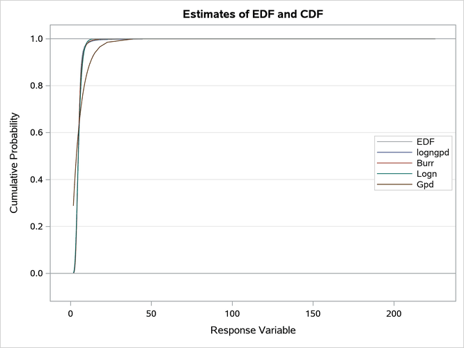
Figure 20: Comparison of the CDF and PDF Estimates of the Fitted Models
 |
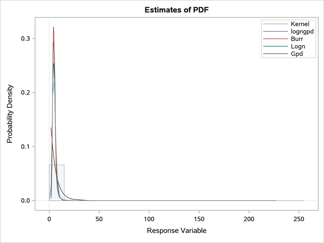 |
The plots in Figure 20 confirm that the GPD distribution fits the data poorly. It is difficult to compare the other three distributions based on the CDF and PDF comparison plots because of the heaviness of the tail. However, the conditional PDF plot in Output 28.3.2 helps you compare the distributions by zooming in on certain regions of the PDF comparison plot.
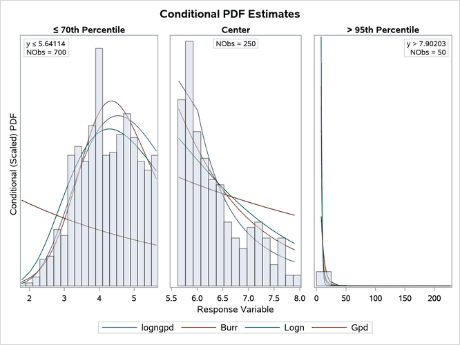
The conditional PDF plot of the left region (' 70th Percentile') shows that Burr and lognormal distributions do not fit the data as well as the LOGNGPD distribution in the body portion. The plot of the center region shows that Burr and lognormal distributions also have a poorer fit in the tail portion than the LOGNGPD distribution. The downward dip in the PDF of the LOGNGPD distribution around y = 6.0 in the center plot shows the approximate location of , where the tail portion of the mixture distribution begins. This illustrates the LOGNGPD distribution’s ability to adapt to the tail.
Output 28.3.2: Comparison of the Conditional PDF Estimates of the Fitted Models
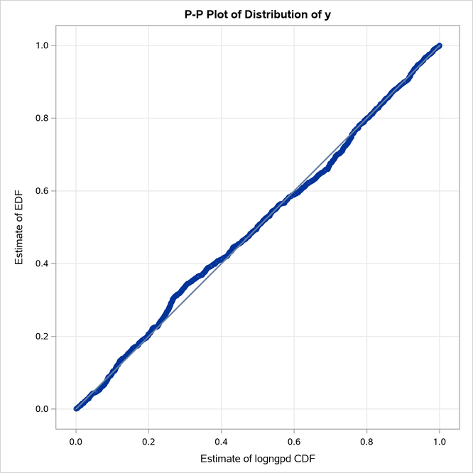
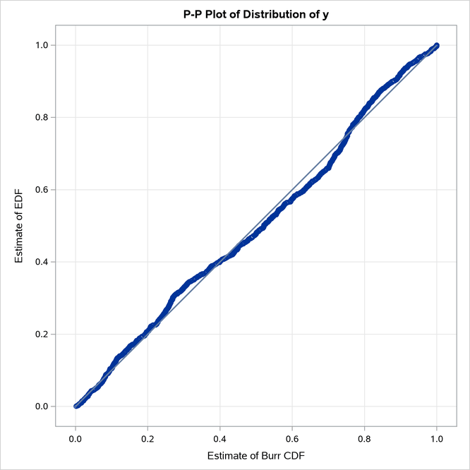
The Burr distribution is the closest contender to the LOGNGPD distribution. The P-P plots in Figure 21 provide more visual confirmation that the LOGNGPD distribution fits the tail region better than the Burr distribution.
Figure 21: P-P Plots for the LOGNGPD and BURR Distribution Models
 |
 |
The detailed results for the LOGNGPD distribution are shown in Output 28.3.3. The initial values table shows the fixed value of the Pn parameter that the LOGNGPD_PARMINIT subroutine sets. The table uses the bounds columns to indicate that it is a constant parameter. The last table in the figure shows the final parameter estimates. The estimates of all free parameters are significantly different from 0. As expected, the final estimate of the constant parameter Pn has not changed from its initial value.
Output 28.3.3: Detailed Results for the LOGNGPD Distribution
| Distribution Information | |
|---|---|
| Name | logngpd |
| Description | Lognormal Body-GPD Tail Distribution. Mu, Sigma, Xi, and Xr are free parameters. Pn is a constant parameter. |
| Distribution Parameters | 5 |
| Initial Parameter Values and Bounds | |||
|---|---|---|---|
| Parameter | Initial Value |
Lower Bound |
Upper Bound |
| Mu | 1.14149 | -Infty | Infty |
| Sigma | 1.03316 | 1.05367E-8 | Infty |
| Xi | 0.48188 | 1.05367E-8 | Infty |
| Xr | 1.62621 | 1.05367E-8 | Infty |
| Pn | 0.80000 | Constant | Constant |
| Convergence Status |
|---|
| Convergence criterion (GCONV=1E-8) satisfied. |
| Optimization Summary | |
|---|---|
| Optimization Technique | Trust Region |
| Iterations | 26 |
| Function Calls | 81 |
| Failed Function Calls | 1 |
| Log Likelihood | -1819.8 |
| Parameter Estimates | |||||
|---|---|---|---|---|---|
| Parameter | DF | Estimate | Standard Error |
t Value | Approx Pr > |t| |
| Mu | 1 | 1.61374 | 0.02509 | 64.31 | <.0001 |
| Sigma | 1 | 0.31716 | 0.01541 | 20.59 | <.0001 |
| Xi | 1 | 0.53177 | 0.08867 | 6.00 | <.0001 |
| Xr | 1 | 1.19816 | 0.03925 | 30.52 | <.0001 |
| Pn | 1 | 0.80000 | Constant | . | . |
The following SAS statements use the parameter estimates to compute the value where the tail region is estimated to start ( ) and the scale of the GPD tail distribution (
 ):
):
/*-------- Compute tail cutoff and tail distribution's scale --------*/
data xb_thetat(keep=x_b theta_t);
   set parmest(where=(_MODEL_='logngpd' and _TYPE_='EST'));
   x_b = exp(Mu) * Xr;
   theta_t = (CDF('LOGN',x_b,Mu,Sigma)/PDF('LOGN',x_b,Mu,Sigma)) *
             ((1-Pn)/Pn);
run;

proc print data=xb_thetat noobs;
run;
Output 28.3.4: Start of the Tail and Scale of the GPD Tail Distribution
| x_b | theta_t |
|---|---|
| 6.01665 | 1.00677 |
The computed values of and are shown as x_b and theta_t in Output 28.3.4. Equipped with this additional derived information, you can now interpret the results of fitting the mixed-tail distribution as follows:
The tail starts at
 . Optimizing the scale-normalized relative cutoff () in addition to optimizing the scale of the body region (
 ) gives you more flexibility in optimizing the absolute cutoff (). If Xr is declared as a constant parameter, then is optimized by virtue of optimizing the scale of the body region (), and you must rely on Hill’s tail index estimator to yield an initial estimate of that is close to an optimal estimate. By keeping Xr as a free parameter, you account for the possibility that Hill’s estimator can yield a suboptimal estimate.
 The values
 follow the lognormal distribution with parameters
  and
and  . These parameter estimates are reasonably close to the parameters of the body distribution that is used for simulating the sample.
 If
 denotes the loss random variable for the tail defined as
  , where X is the original loss variable, then for this example,
  follows the GPD density function with scale
  and shape
  .
.