Regression Action Set
The logistic Action
Binary Logistic Regression
(View the complete code for this example.)
This section contains PROC CAS code.
Note: Input data must be accessible in your CAS session, either as a CAS table or as a transient-scope table. A CAS table has a two-level name: the first level is your CAS engine libref, and the second level is the table name. You refer to this table in the CAS procedure by specifying only the second level. For more information about two-level names, see Chapter 2, Shared Concepts. A transient-scope table is called directly from the action and exists in memory for the duration of the action. For more information about accessing data, see SAS Viya: System Programming Guide. For more information about PROC CAS and programming in CASL, see SAS Cloud Analytic Services: CASL Programmer’s Guide and SAS Cloud Analytic Services: CASL Reference.
The following DATA step creates the getStarted data table, which consists of 1,000 observations on a dichotomous response variable (y), a character variable (C), and 10 numeric variables (x1–x10).
proc cas;
dataStep.runCode /
    code="
   data getStarted;
      nTotalObs=1000;
      drop c2 eta pr i rew nTotalObs nObsPerThread nExtras;
      call streaminit(1);
      nObsPerThread = int(nTotalObs/_nthreads_);
      nExtras       = mod(nTotalObs,_nthreads_);
      if _threadid_ <= nExtras then nObsPerThread = nObsPerThread + 1;
      do i=1 to nObsPerThread;
         id = (_threadid_ - 1) * nObsPerThread + i;
         if _threadid_ > nExtras then id = id + nExtras;
         rew = rand('rewind', id);
         x1=round(rand('normal')*5+10,.1); x2=round(7*rand('uniform'))/7;
         x3=round(rand('normal')*1+2,.1);  x4=round(50*rand('uniform'));
         x5=round(100*rand('uniform'));    x6=round(rand('normal')*.8+1.5,.1);
         x7=10*round(10*rand('uniform'));  x8=round(10*rand('uniform'))/10;
         x9=round(rand('normal')*3+5,.1);  x10=round(rand('normal')*2+3,.1);
         c2=rand('uniform');
         if      (c2<.1) then C='A'; else if (c2<.2) then C='B';
         else if (c2<.3) then C='C'; else if (c2<.4) then C='D';
         else if (c2<.5) then C='E'; else if (c2<.6) then C='F';
         else if (c2<.7) then C='G'; else if (c2<.8) then C='H';
         else if (c2<.9) then C='I'; else                 C='J';
         eta=1-x2-x8;
         pr= exp(eta)/(1+exp(eta));
         y=(rand('uniform') > pr);
         output;
      end;
   run;
   ",
    single="no";
run;
By default, the CAS server executes the preceding DATA step in parallel in every thread on every node in your session. For example, if your DATA step creates 10 observations and executes in parallel on a session that has three worker nodes each of which uses 16 threads, then the resulting CAS table has 160 observations on each worker node, yielding a CAS table with a total of 480 observations. The preceding DATA step uses this technique to create a table with a specified number of observations in parallel on your CAS server by dividing the desired number of observations (nTotalObs) by the total number of threads (_nthreads_). If the number of observations cannot be exactly divided by the number of threads, the code adds one observation to each of a subset of the threads until all observations are accounted for.
The following statements use the logistic action in the regression action set to fit a logistic model to these data. The table parameter names the input data table to be analyzed. The class parameter specifies that the variable C is a classification variable; this parameter corresponds to the CLASS statement in the LOGSELECT procedure. The model parameter specifies the model: the depvars subparameter specifies the variable y as the response variable, and the effects subparameter lists the classification variable C and the 10 numeric explanatory variables, x1–x10. The itHist subparameter in the optimization parameter list produces a table that summarizes the steps of the optimization. The outputTables parameter outputs the fitted parameter estimates to the mycas.pe data table.
proc cas;
regression.logistic /
    class={"C"},
    model={depvar="y",
           effects={"C", "x1", "x2", "x3", "x4", "x5", "x6", "x7", "x8", "x9",
                    "x10"}},
    optimization={itHist="summary"},
    outputTables={names={parameterestimates="pe"}},
    table="getStarted";
run;
The output from this analysis is displayed by default, and is presented in Output 22.5.1 through Output 22.5.10.
Output 22.5.1 displays the "Model Information" table. The logistic action uses a Newton-Raphson algorithm to model a binary distribution with a logit link function for the variable y.
Output 22.5.1: Model Information
| Model Information | |
|---|---|
| Data Source | GETSTARTED |
| Response Variable | y |
| Distribution | Binary |
| Link Function | Logit |
| Optimization Technique | Newton-Raphson with Ridging |
Output 22.5.2 displays the "Number of Observations" table. All 1,000 observations in the data table are used in the analysis.
Output 22.5.2: Number of Observations
| Number of Observations Read | 1000 |
|---|---|
| Number of Observations Used | 1000 |
The "Response Profile" table in Output 22.5.3 shows the breakdown of the response variable levels by frequency. By default for binary data, the logistic action models the probability of the event with the lower-ordered value in the "Response Profile" table, as indicated by the note that follows the table. (You can use the response-variable subparameters in the model parameter to choose which value of the response variable to model.) In this example, the values that are represented by y = 0 are modeled as the "successes" in the Bernoulli experiments.
Output 22.5.3: Response Profile
| Response Profile | ||
|---|---|---|
| Ordered Value |
y | Total Frequency |
| 1 | 0 | 484 |
| 2 | 1 | 516 |
| Probability modeled is y = 0. |
The classification variable C has 10 unique formatted levels that are displayed in the "Class Level Information" table in Output 22.5.4.
Output 22.5.4: Class Level Information
| Class Level Information | ||
|---|---|---|
| Class | Levels | Values |
| C | 10 | A B C D E F G H I J |
The "Iteration History" table is shown in Output 22.5.5. The Newton-Raphson algorithm with ridging converged after three iterations, not counting the initial setup iteration.
Output 22.5.5: Iteration History
| Iteration History | ||||
|---|---|---|---|---|
| Iteration | Evaluations | Objective Function |
Change | Maximum Gradient |
| 0 | 4 | 0.6613855981 | 0.20692 | |
| 1 | 2 | 0.6583727872 | 0.00301281 | 0.01883 |
| 2 | 2 | 0.6583596409 | 0.00001315 | 0.000082 |
| 3 | 2 | 0.6583596407 | 0.00000000 | 1.23E-9 |
Output 22.5.6 displays the final convergence status of the Newton-Raphson algorithm. The gconv relative convergence criterion is satisfied.
Output 22.5.6: Convergence Status
| Convergence criterion (GCONV=1E-8) satisfied. |
Output 22.5.7 displays the "Dimensions" table for this model. This table summarizes some important sizes of various model components. For example, it shows that the design matrix  has 21 columns, which correspond to 1 column for the intercept, 10 columns for the effect associated with the classification variable
 C, and 1 column each for the continuous variables x1–x10. However, the rank of the crossproducts matrix is only 20. Because the classification variable C uses GLM parameterization and because the model contains an intercept, there is one singularity in the crossproducts matrix of the model. Consequently, only 20 parameters enter the optimization.
Output 22.5.7: Dimensions in Binomial Logistic Regression
| Dimensions | |
|---|---|
| Columns in Design | 21 |
| Number of Effects | 12 |
| Max Effect Columns | 10 |
| Rank of Design | 20 |
| Parameters in Optimization | 20 |
Output 22.5.8 shows the global test for the null hypothesis that all model effects jointly do not affect the probability of success of the binary response. The test is significant (p < 0.0001). One or more of the model effects thus significantly affect the probability of observing an event.
Output 22.5.8: Null Test
| Testing Global Null Hypothesis: BETA=0 | |||
|---|---|---|---|
| Test | DF | Chi-Square | Pr > ChiSq |
| Likelihood Ratio | 19 | 68.5509 | <.0001 |
The "Fit Statistics" table is shown in Output 22.5.9. The –2 log likelihood at the converged estimates is 1,316.7. You can use this value to compare the model to nested model alternatives by means of a likelihood ratio test. To compare models that are not nested, you can use information criteria such as AIC (Akaike’s information criterion), AICC (Akaike’s bias-corrected information criterion), and SBC (Schwarz Bayesian information criterion). These criteria penalize the –2 log likelihood for the number of parameters. Because of the large number of parameters, the discrepancy between the –2 log likelihood and AIC (for example) is substantial in this case.
Output 22.5.9: Fit Statistics
| Fit Statistics | |
|---|---|
| -2 Log Likelihood | 1316.71928 |
| AIC (smaller is better) | 1356.71928 |
| AICC (smaller is better) | 1357.57730 |
| SBC (smaller is better) | 1454.87439 |
However, the "Parameter Estimates" table in Output 22.5.10 shows that many parameters have fairly large p-values, indicating that one or more of the model effects might not be necessary.
Output 22.5.10: Parameter Estimates
| Parameter Estimates | |||||
|---|---|---|---|---|---|
| Parameter | DF | Estimate | Standard Error |
Chi-Square | Pr > ChiSq |
| Intercept | 1 | 0.091372 | 0.419472 | 0.0474 | 0.8276 |
| C A | 1 | 0.101855 | 0.295610 | 0.1187 | 0.7304 |
| C B | 1 | 0.313845 | 0.289155 | 1.1781 | 0.2778 |
| C C | 1 | 0.514901 | 0.288989 | 3.1746 | 0.0748 |
| C D | 1 | 0.190620 | 0.307220 | 0.3850 | 0.5350 |
| C E | 1 | 0.115930 | 0.285505 | 0.1649 | 0.6847 |
| C F | 1 | 0.488200 | 0.292348 | 2.7887 | 0.0949 |
| C G | 1 | 0.607139 | 0.290986 | 4.3534 | 0.0369 |
| C H | 1 | 0.422393 | 0.286422 | 2.1748 | 0.1403 |
| C I | 1 | 0.099037 | 0.284288 | 0.1214 | 0.7276 |
| C J | 0 | 0 | . | . | . |
| x1 | 1 | 0.000629 | 0.013073 | 0.0023 | 0.9616 |
| x2 | 1 | -1.133344 | 0.228116 | 24.6838 | <.0001 |
| x3 | 1 | 0.077254 | 0.065331 | 1.3983 | 0.2370 |
| x4 | 1 | 0.001466 | 0.004652 | 0.0993 | 0.7526 |
| x5 | 1 | 0.003207 | 0.002301 | 1.9414 | 0.1635 |
| x6 | 1 | 0.041222 | 0.083063 | 0.2463 | 0.6197 |
| x7 | 1 | -0.001533 | 0.002237 | 0.4694 | 0.4933 |
| x8 | 1 | -1.063694 | 0.232968 | 20.8469 | <.0001 |
| x9 | 1 | 0.015834 | 0.022353 | 0.5018 | 0.4787 |
| x10 | 1 | 0.074454 | 0.033162 | 5.0408 | 0.0248 |
Finally, the procedure displays the table in Output 22.5.11, which shows the amount of time (in seconds) that the logistic action spent on different tasks in the analysis.
Output 22.5.11: Procedure Timing
| Task Timing | ||
|---|---|---|
| Task | Seconds | Percent |
| Setup and Parsing | 0.02 | 25.64% |
| Levelization | 0.01 | 14.43% |
| Model Initialization | 0.00 | 5.35% |
| SSCP Computation | 0.01 | 18.15% |
| Model Fitting | 0.03 | 34.89% |
| Cleanup | 0.00 | 0.01% |
| Total | 0.08 | 100.00% |
Output 22.5.10 shows that the full model has many nonsignificant effects. You can perform forward selection on these data by using the following statements. Effects that provide the best improvement for the default selection criterion, SBC, are added until no more effects can improve the selection criterion. The method subparameter in the selection parameter enables you to choose the selection method, and the details subparameter produces all tables that are related to model selection. The traceNames subparameter in the display parameter displays the full pathnames of the output tables (not shown here).
proc cas;
regression.logistic /
    class={"C"},
    display={traceNames="true"},
    model={depvar="y",
           effects={"C", "x1", "x2", "x3", "x4", "x5", "x6", "x7", "x8", "x9",
                    "x10"}},
    selection={details="all", method="forward"},
    table="getStarted";
run;
The model selection tables are shown in Output 22.5.12 through Output 22.5.14. Results from the selected model are shown in Output 22.5.15 and Output 22.5.16.
The "Selection Information" table in Output 22.5.12 summarizes the settings for the model selection. At each step, an effect is added to the model only if it produces the most significant improvement in the SBC. The forward selection stops three steps after the smallest SBC is obtained, or when all effects have been added to the model.
Output 22.5.12: Selection Information
| Selection Information | |
|---|---|
| Selection Method | Forward |
| Select Criterion | SBC |
| Stop Criterion | SBC |
| Effect Hierarchy Enforced | None |
| Stop Horizon | 3 |
For each step of the selection process, the details=all subparameter displays the effects that are candidates for entering the model along with their selection criterion (SBC). Output 22.5.13 displays this table for the first step; the other steps are not shown here.
Output 22.5.13: Best 10 Entry Candidates for Step 1
| Best 10 Entry Candidates | ||
|---|---|---|
| Rank | Effect | SBC |
| 1 | x2 | 1370.7425 |
| 2 | x8 | 1377.1766 |
| 3 | x10 | 1393.3327 |
| 4 | x3 | 1397.3647 |
| 5 | x5 | 1398.2532 |
| 6 | x6 | 1398.5991 |
| 7 | x4 | 1398.6078 |
| 8 | x9 | 1398.7225 |
| 9 | x7 | 1398.9572 |
| 10 | x1 | 1399.0848 |
The details=all subparameter also displays the dimensions, global test, fit statistics, and parameter estimates at each step of the selection process; these details are not shown here.
When the selection procedure is complete, the "Selection Summary" table in Output 22.5.14 shows the effects that were added to the model and the value of their selection criterion (and the choose and stop criteria, if they are specified). Step 0 refers to the null model that contains only an intercept. In step 1, effect x8 made the most significant contribution to the model among the candidate effects, according to the SBC statistic. In step 2, x2 made the most significant contribution when an effect was added to a model that contains the intercept and x8. In the three subsequent steps, no effect could be added to the model that would reduce the SBC, so variable selection stopped because the stop horizon indicates that at most three steps beyond the minimum SBC value are to be taken (see Output 22.5.12) .
In Output 22.5.14, the "Selection Summary" table is followed by three small tables that summarize why the process stopped and which model is selected.
Output 22.5.14: Selection Summary Information
| Selection Summary | |||
|---|---|---|---|
| Step | Effect Entered |
Number Effects In |
SBC |
| 0 | Intercept | 1 | 1392.1779 |
| 1 | x2 | 2 | 1370.7425 |
| 2 | x8 | 3 | 1356.8279* |
| 3 | x10 | 4 | 1358.3616 |
| 4 | x3 | 5 | 1363.5113 |
| 5 | x5 | 6 | 1368.8719 |
| * Optimal Value Of Criterion | |||
Output 22.5.15 displays information about the selected model. Notice that the –2 log-likelihood value in the "Fit Statistics" table is larger than the value for the full model in Output 22.5.9. This is expected because the selected model contains only a subset of the parameters. Because the selected model is more parsimonious than the full model, the discrepancy between the –2 log likelihood and the information criteria is less severe than previously noted.
Output 22.5.15: Fit Statistics and Null Test
| Dimensions | |
|---|---|
| Columns in Design | 3 |
| Number of Effects | 3 |
| Max Effect Columns | 1 |
| Rank of Design | 3 |
| Parameters in Optimization | 3 |
The parameter estimates of the selected model are shown in Output 22.5.16. Notice that the effects are listed in the "Parameter Estimates" table in the order in which they were specified in the model parameter and not in the order in which they were added to the model.
Output 22.5.16: Parameter Estimates
| Parameter Estimates | |||||
|---|---|---|---|---|---|
| Parameter | DF | Estimate | Standard Error |
Chi-Square | Pr > ChiSq |
| Intercept | 1 | 1.004603 | 0.169966 | 34.9353 | <.0001 |
| x2 | 1 | -1.151380 | 0.223567 | 26.5231 | <.0001 |
| x8 | 1 | -1.030894 | 0.228869 | 20.2887 | <.0001 |
You can construct the prediction equation for this model from the parameter estimates as follows. The estimated linear predictor for an observation is

The predicted probability that variable y takes the value 0 is

Binary Logistic Regression
(View the complete code for this example.)
This section contains Lua code that creates the same getStarted table and performs the same analysis as shown in the CASL version of this example. For more information about coding in Lua, see Getting Started with SAS Viya for Lua and SAS Viya: System Programming Guide.
Because this example uses simulated data that are produced from DATA step code, you can submit the runCode action on your Lua client to create the simulated data in your CAS session. The following DATA step creates the getStarted data table, which consists of 1,000 observations on a dichotomous response variable (y), a character variable (C), and 10 numeric variables (x1–x10).
s:dataStep_runCode{single='no', code=[[
data getStarted;
   nTotalObs=1000;
   drop c2 eta pr i rew nTotalObs nObsPerThread nExtras;
   call streaminit(1);
   nObsPerThread = int(nTotalObs/_nthreads_);
   nExtras       = mod(nTotalObs,_nthreads_);
   if _threadid_ <= nExtras then nObsPerThread = nObsPerThread + 1;
   do i=1 to nObsPerThread;
      id = (_threadid_ - 1) * nObsPerThread + i;
      if _threadid_ > nExtras then id = id + nExtras;
      rew = rand('rewind', id);
      x1=round(rand('normal')*5+10,.1); x2=round(7*rand('uniform'))/7;
      x3=round(rand('normal')*1+2,.1);  x4=round(50*rand('uniform'));
      x5=round(100*rand('uniform'));    x6=round(rand('normal')*.8+1.5,.1);
      x7=10*round(10*rand('uniform'));  x8=round(10*rand('uniform'))/10;
      x9=round(rand('normal')*3+5,.1);  x10=round(rand('normal')*2+3,.1);
      c2=rand('uniform');
      if      (c2<.1) then C='A'; else if (c2<.2) then C='B';
      else if (c2<.3) then C='C'; else if (c2<.4) then C='D';
      else if (c2<.5) then C='E'; else if (c2<.6) then C='F';
      else if (c2<.7) then C='G'; else if (c2<.8) then C='H';
      else if (c2<.9) then C='I'; else                 C='J';
      eta=1-x2-x8;
      pr= exp(eta)/(1+exp(eta));
      y=(rand('uniform') > pr);
      output;
   end;
run;
]] }
By default, the CAS server executes the preceding DATA step in parallel in every thread on every node in your session. For example, if your DATA step creates 10 observations and executes in parallel on a session that has three worker nodes each of which uses 16 threads, then the resulting CAS table has 160 observations on each worker node, yielding a CAS table with a total of 480 observations. The preceding DATA step uses this technique to create a table with a specified number of observations in parallel on your CAS server by dividing the desired number of observations (nTotalObs) by the total number of threads (_nthreads_). If the number of observations cannot be exactly divided by the number of threads, the code adds one observation to each of a subset of the threads until all observations are accounted for.
The following statements use the logistic action in the regression action set to fit a logistic model to these data. The table parameter names the input data table to be analyzed. The class parameter specifies that the variable C is a classification variable; this parameter corresponds to the CLASS statement in the LOGSELECT procedure. The model parameter specifies the model: the depvars subparameter specifies the variable y as the response variable, and the effects subparameter lists the classification variable C and the 10 numeric explanatory variables, x1–x10. The itHist subparameter in the optimization parameter list produces a table that summarizes the steps of the optimization. The outputTables parameter outputs the fitted parameter estimates to the pe data table.
s:loadactionset{actionset="regression"}
s:regression_logistic{
   table='getStarted',
   class={'C'},
   model={depvar='y',
          effects={'C', 'x1', 'x2', 'x3', 'x4', 'x5',
                   'x6', 'x7', 'x8', 'x9', 'x10'}},
   optimization={itHist='summary'},
   outputTables={names={parameterestimates='pe'}} }
The output from this analysis is displayed by default, and is presented in Output 22.5.17 through Output 22.5.26.
Output 22.5.17 displays the "Model Information" table. The logistic action uses a Newton-Raphson algorithm to model a binary distribution with a logit link function for the variable y.
Output 22.5.17: Model Information
| RowId | Description | Value |
|---|---|---|
| DATA | Data Source | GETSTARTED |
| RESPONSEVAR | Response Variable | y |
| DIST | Distribution | Binary |
| LINK | Link Function | Logit |
| TECH | Optimization Technique | Newton-Raphson with Ridging |
Output 22.5.18 displays the "Number of Observations" table. All 1,000 observations in the data table are used in the analysis.
Output 22.5.18: Number of Observations
| RowId | Description | Value |
|---|---|---|
| NREAD | Number of Observations Read | 1000 |
| NUSED | Number of Observations Used | 1000 |
The "Response Profile" table in Output 22.5.19 shows the breakdown of the response variable levels by frequency. By default for binary data, the logistic action models the probability of the event with the lower-ordered value in the "Response Profile" table, as indicated by the note that follows the table. (You can use the response-variable subparameters in the model parameter to choose which value of the response variable to model.) In this example, the values that are represented by y = 0 are modeled as the "successes" in the Bernoulli experiments.
Output 22.5.19: Response Profile
| OrderedValue | Outcome | y | Freq | Modeled |
|---|---|---|---|---|
| 1 | 0 | 0 | 484 | * |
| 2 | 1 | 1 | 516 |
The classification variable C has 10 unique formatted levels that are displayed in the "Class Level Information" table in Output 22.5.20.
Output 22.5.20: Class Level Information
| Class | Levels | Values |
|---|---|---|
| C | 10 | A B C D E F G H I J |
The "Iteration History" table is shown in Output 22.5.21. The Newton-Raphson algorithm with ridging converged after three iterations, not counting the initial setup iteration.
Output 22.5.21: Iteration History
| Iteration | Evaluations | Objective | Change | MaxGradient |
|---|---|---|---|---|
| 0 | 4 | 0.6613855981 | _ | 0.20692 |
| 1 | 2 | 0.6583727872 | 0.00301281 | 0.01883 |
| 2 | 2 | 0.6583596409 | 0.00001315 | 0.000082 |
| 3 | 2 | 0.6583596407 | 0.00000000 | 1.23E-9 |
Output 22.5.22 displays the final convergence status of the Newton-Raphson algorithm. The gconv relative convergence criterion is satisfied.
Output 22.5.22: Convergence Status
| Reason | Status | MaxGradient | Separation |
|---|---|---|---|
| Convergence criterion (GCONV=1E-8) satisfied. | 0 | 1.23E-9 | 0 |
Output 22.5.23 displays the "Dimensions" table for this model. This table summarizes some important sizes of various model components. For example, it shows that the design matrix has 21 columns, which correspond to 1 column for the intercept, 10 columns for the effect associated with the classification variable C, and 1 column each for the continuous variables x1–x10. However, the rank of the crossproducts matrix is only 20. Because the classification variable C uses GLM parameterization and because the model contains an intercept, there is one singularity in the crossproducts matrix of the model. Consequently, only 20 parameters enter the optimization.
Output 22.5.23: Dimensions in Binomial Logistic Regression
| RowId | Description | Value |
|---|---|---|
| NDESIGNCOLS | Columns in Design | 21 |
| NEFFECTS | Number of Effects | 12 |
| MAXEFCOLS | Max Effect Columns | 10 |
| DESIGNRANK | Rank of Design | 20 |
| OPTPARM | Parameters in Optimization | 20 |
Output 22.5.24 shows the global test for the null hypothesis that all model effects jointly do not affect the probability of success of the binary response. The test is significant (p < 0.0001). One or more of the model effects thus significantly affect the probability of observing an event.
Output 22.5.24: Null Test
| Test | DF | ChiSq | ProbChiSq |
|---|---|---|---|
| Likelihood Ratio | 19 | 68.5509 | <.0001 |
The "Fit Statistics" table is shown in Output 22.5.25. The –2 log likelihood at the converged estimates is 1,316.7. You can use this value to compare the model to nested model alternatives by means of a likelihood ratio test. To compare models that are not nested, you can use information criteria such as AIC (Akaike’s information criterion), AICC (Akaike’s bias-corrected information criterion), and SBC (Schwarz Bayesian information criterion). These criteria penalize the –2 log likelihood for the number of parameters. Because of the large number of parameters, the discrepancy between the –2 log likelihood and AIC (for example) is substantial in this case.
Output 22.5.25: Fit Statistics
| RowId | Description | Value |
|---|---|---|
| M2LL | -2 Log Likelihood | 1316.71928 |
| AIC | AIC (smaller is better) | 1356.71928 |
| AICC | AICC (smaller is better) | 1357.57730 |
| SBC | SBC (smaller is better) | 1454.87439 |
However, the "Parameter Estimates" table in Output 22.5.26 shows that many parameters have fairly large p-values, indicating that one or more of the model effects might not be necessary.
Output 22.5.26: Parameter Estimates
| Effect | C | Parameter | ParmName | DF | Estimate | StdErr | ChiSq | ProbChiSq |
|---|---|---|---|---|---|---|---|---|
| Intercept | Intercept | Intercept | 1 | 0.091372 | 0.419472 | 0.0474 | 0.8276 | |
| C | A | C A | C_A | 1 | 0.101855 | 0.295610 | 0.1187 | 0.7304 |
| C | B | C B | C_B | 1 | 0.313845 | 0.289155 | 1.1781 | 0.2778 |
| C | C | C C | C_C | 1 | 0.514901 | 0.288989 | 3.1746 | 0.0748 |
| C | D | C D | C_D | 1 | 0.190620 | 0.307220 | 0.3850 | 0.5350 |
| C | E | C E | C_E | 1 | 0.115930 | 0.285505 | 0.1649 | 0.6847 |
| C | F | C F | C_F | 1 | 0.488200 | 0.292348 | 2.7887 | 0.0949 |
| C | G | C G | C_G | 1 | 0.607139 | 0.290986 | 4.3534 | 0.0369 |
| C | H | C H | C_H | 1 | 0.422393 | 0.286422 | 2.1748 | 0.1403 |
| C | I | C I | C_I | 1 | 0.099037 | 0.284288 | 0.1214 | 0.7276 |
| C | J | C J | C_J | 0 | 0 | . | . | . |
| x1 | x1 | x1 | 1 | 0.000629 | 0.013073 | 0.0023 | 0.9616 | |
| x2 | x2 | x2 | 1 | -1.133344 | 0.228116 | 24.6838 | <.0001 | |
| x3 | x3 | x3 | 1 | 0.077254 | 0.065331 | 1.3983 | 0.2370 | |
| x4 | x4 | x4 | 1 | 0.001466 | 0.004652 | 0.0993 | 0.7526 | |
| x5 | x5 | x5 | 1 | 0.003207 | 0.002301 | 1.9414 | 0.1635 | |
| x6 | x6 | x6 | 1 | 0.041222 | 0.083063 | 0.2463 | 0.6197 | |
| x7 | x7 | x7 | 1 | -0.001533 | 0.002237 | 0.4694 | 0.4933 | |
| x8 | x8 | x8 | 1 | -1.063694 | 0.232968 | 20.8469 | <.0001 | |
| x9 | x9 | x9 | 1 | 0.015834 | 0.022353 | 0.5018 | 0.4787 | |
| x10 | x10 | x10 | 1 | 0.074454 | 0.033162 | 5.0408 | 0.0248 |
Finally, the procedure displays the table in Output 22.5.27, which shows the amount of time (in seconds) that the logistic action spent on different tasks in the analysis.
Output 22.5.27: Procedure Timing
| RowId | Task | Time | RelTime |
|---|---|---|---|
| SETUP | Setup and Parsing | 0.02 | 25.64% |
| LEVELIZATION | Levelization | 0.01 | 14.43% |
| INITIALIZATION | Model Initialization | 0.00 | 5.35% |
| SSCP | SSCP Computation | 0.01 | 18.15% |
| FITTING | Model Fitting | 0.03 | 34.89% |
| CLEANUP | Cleanup | 0.00 | 0.01% |
| TOTAL | Total | 0.08 | 100.00% |
Output 22.5.26 shows that the full model has many nonsignificant effects. You can perform forward selection on these data by using the following statements. Effects that provide the best improvement for the default selection criterion, SBC, are added until no more effects can improve the selection criterion. The method subparameter in the selection parameter enables you to choose the selection method, and the details subparameter produces all tables that are related to model selection. The traceNames subparameter in the display parameter displays the full pathnames of the output tables (not shown here).
s:regression_logistic{
   table='getStarted',
   class={'C'},
   model={depvar='y',
          effects={'C', 'x1', 'x2', 'x3', 'x4', 'x5',
                   'x6', 'x7', 'x8', 'x9', 'x10'}},
   selection={method='forward', details='all'},
   display={traceNames=true} }
The model selection tables are shown in Output 22.5.28 through Output 22.5.30. Results from the selected model are shown in Output 22.5.31 and Output 22.5.32.
The "Selection Information" table in Output 22.5.28 summarizes the settings for the model selection. At each step, an effect is added to the model only if it produces the most significant improvement in the SBC. The forward selection stops three steps after the smallest SBC is obtained, or when all effects have been added to the model.
Output 22.5.28: Selection Information
| RowId | Description | Value | NValue |
|---|---|---|---|
| METHOD | Selection Method | Forward | _ |
| SELCRITERION | Select Criterion | SBC | _ |
| STOPCRITERION | Stop Criterion | SBC | _ |
| HIERARCHY | Effect Hierarchy Enforced | None | _ |
| STOPHORIZON | Stop Horizon | 3 | 3 |
For each step of the selection process, the details=all subparameter displays the effects that are candidates for entering the model along with their selection criterion (SBC). Output 22.5.29 displays this table for the first step; the other steps are not shown here.
Output 22.5.29: Best 10 Entry Candidates for Step 1
| Step | Rank | Effect | SBC |
|---|---|---|---|
| 1 | 1 | x2 | 1370.7425 |
| 1 | 2 | x8 | 1377.1766 |
| 1 | 3 | x10 | 1393.3327 |
| 1 | 4 | x3 | 1397.3647 |
| 1 | 5 | x5 | 1398.2532 |
| 1 | 6 | x6 | 1398.5991 |
| 1 | 7 | x4 | 1398.6078 |
| 1 | 8 | x9 | 1398.7225 |
| 1 | 9 | x7 | 1398.9572 |
| 1 | 10 | x1 | 1399.0848 |
The details=all subparameter also displays the dimensions, global test, fit statistics, and parameter estimates at each step of the selection process; these details are not shown here.
When the selection procedure is complete, the "Selection Summary" table in Output 22.5.30 shows the effects that were added to the model and the value of their selection criterion (and the choose and stop criteria, if they are specified). Step 0 refers to the null model that contains only an intercept. In step 1, effect x8 made the most significant contribution to the model among the candidate effects, according to the SBC statistic. In step 2, x2 made the most significant contribution when an effect was added to a model that contains the intercept and x8. In the three subsequent steps, no effect could be added to the model that would reduce the SBC, so variable selection stopped because the stop horizon indicates that at most three steps beyond the minimum SBC value are to be taken (see Output 22.5.28) .
In Output 22.5.30, the "Selection Summary" table is followed by three small tables that summarize why the process stopped and which model is selected.
Output 22.5.30: Selection Summary Information
| Control | Step | EffectEntered | nEffectsIn | SBC | OptSBC |
|---|---|---|---|---|---|
| 0 | Intercept | 1 | 1392.1779 | 0 | |
| - | 1 | x2 | 2 | 1370.7425 | 0 |
| 2 | x8 | 3 | 1356.8279 | 1 | |
| 3 | x10 | 4 | 1358.3616 | 0 | |
| 4 | x3 | 5 | 1363.5113 | 0 | |
| 5 | x5 | 6 | 1368.8719 | 0 |
| Reason | Code |
|---|---|
| Selection stopped at a local minimum of the STOP criterion. | 6 |
| Reason |
|---|
| The model at step 2 is selected. |
| Label | Effects |
|---|---|
| Selected Effects: | Intercept x2 x8 |
Output 22.5.31 displays information about the selected model. Notice that the –2 log-likelihood value in the "Fit Statistics" table is larger than the value for the full model in Output 22.5.25. This is expected because the selected model contains only a subset of the parameters. Because the selected model is more parsimonious than the full model, the discrepancy between the –2 log likelihood and the information criteria is less severe than previously noted.
Output 22.5.31: Fit Statistics and Null Test
| Step | RowId | Description | Value |
|---|---|---|---|
| S | NDESIGNCOLS | Columns in Design | 3 |
| S | NEFFECTS | Number of Effects | 3 |
| S | MAXEFCOLS | Max Effect Columns | 1 |
| S | DESIGNRANK | Rank of Design | 3 |
| S | OPTPARM | Parameters in Optimization | 3 |
| Step | Test | DF | ChiSq | ProbChiSq |
|---|---|---|---|---|
| S | Likelihood Ratio | 2 | 49.2731 | <.0001 |
| Step | RowId | Description | Value |
|---|---|---|---|
| S | M2LL | -2 Log Likelihood | 1335.99712 |
| S | AIC | AIC (smaller is better) | 1341.99712 |
| S | AICC | AICC (smaller is better) | 1342.02122 |
| S | SBC | SBC (smaller is better) | 1356.72038 |
The parameter estimates of the selected model are shown in Output 22.5.32. Notice that the effects are listed in the "Parameter Estimates" table in the order in which they were specified in the model parameter and not in the order in which they were added to the model.
Output 22.5.32: Parameter Estimates
| Step | Effect | Parameter | ParmName | DF | Estimate | StdErr | ChiSq | ProbChiSq |
|---|---|---|---|---|---|---|---|---|
| S | Intercept | Intercept | Intercept | 1 | 1.004603 | 0.169966 | 34.9353 | <.0001 |
| S | x2 | x2 | x2 | 1 | -1.151380 | 0.223567 | 26.5231 | <.0001 |
| S | x8 | x8 | x8 | 1 | -1.030894 | 0.228869 | 20.2887 | <.0001 |
You can construct the prediction equation for this model from the parameter estimates as follows. The estimated linear predictor for an observation is
The predicted probability that variable y takes the value 0 is
Binary Logistic Regression
(View the complete code for this example.)
This section contains Python code that creates the same getStarted table and performs the same analysis as shown in the CASL version of this example. For more information about coding in Python, see Getting Started with SAS Viya for Python and SAS Viya: System Programming Guide.
Because this example uses simulated data that are produced from DATA step code, you can submit the runCode action on your Python client to create the simulated data in your CAS session. The following DATA step creates the getStarted data table, which consists of 1,000 observations on a dichotomous response variable (y), a character variable (C), and 10 numeric variables (x1–x10).
s.datastep.runcode(
    code='''
   data getStarted;
      nTotalObs=1000;
      drop c2 eta pr i rew nTotalObs nObsPerThread nExtras;
      call streaminit(1);
      nObsPerThread = int(nTotalObs/_nthreads_);
      nExtras       = mod(nTotalObs,_nthreads_);
      if _threadid_ <= nExtras then nObsPerThread = nObsPerThread + 1;
      do i=1 to nObsPerThread;
         id = (_threadid_ - 1) * nObsPerThread + i;
         if _threadid_ > nExtras then id = id + nExtras;
         rew = rand('rewind', id);
         x1=round(rand('normal')*5+10,.1); x2=round(7*rand('uniform'))/7;
         x3=round(rand('normal')*1+2,.1);  x4=round(50*rand('uniform'));
         x5=round(100*rand('uniform'));    x6=round(rand('normal')*.8+1.5,.1);
         x7=10*round(10*rand('uniform'));  x8=round(10*rand('uniform'))/10;
         x9=round(rand('normal')*3+5,.1);  x10=round(rand('normal')*2+3,.1);
         c2=rand('uniform');
         if      (c2<.1) then C='A'; else if (c2<.2) then C='B';
         else if (c2<.3) then C='C'; else if (c2<.4) then C='D';
         else if (c2<.5) then C='E'; else if (c2<.6) then C='F';
         else if (c2<.7) then C='G'; else if (c2<.8) then C='H';
         else if (c2<.9) then C='I'; else                 C='J';
         eta=1-x2-x8;
         pr= exp(eta)/(1+exp(eta));
         y=(rand('uniform') > pr);
         output;
      end;
   run;
   ''',
    single='no')
By default, the CAS server executes the preceding DATA step in parallel in every thread on every node in your session. For example, if your DATA step creates 10 observations and executes in parallel on a session that has three worker nodes each of which uses 16 threads, then the resulting CAS table has 160 observations on each worker node, yielding a CAS table with a total of 480 observations. The preceding DATA step uses this technique to create a table with a specified number of observations in parallel on your CAS server by dividing the desired number of observations (nTotalObs) by the total number of threads (_nthreads_). If the number of observations cannot be exactly divided by the number of threads, the code adds one observation to each of a subset of the threads until all observations are accounted for.
The following statements use the logistic action in the regression action set to fit a logistic model to these data. The table parameter names the input data table to be analyzed. The class parameter specifies that the variable C is a classification variable; this parameter corresponds to the CLASS statement in the LOGSELECT procedure. The model parameter specifies the model: the depvars subparameter specifies the variable y as the response variable, and the effects subparameter lists the classification variable C and the 10 numeric explanatory variables, x1–x10. The itHist subparameter in the optimization parameter list produces a table that summarizes the steps of the optimization. The outputTables parameter outputs the fitted parameter estimates to the pe data table.
s.loadactionset(actionset='regression')
s.regression.logistic(
    class_=['C'],
    model=dict(depvar='y',
               effects=['C', 'x1', 'x2', 'x3', 'x4', 'x5', 'x6', 'x7', 'x8',
                        'x9', 'x10']),
    optimization=dict(itHist='summary'),
    outputTables=dict(names=dict(parameterestimates='pe')),
    table='getStarted')
The output from this analysis is displayed by default, and is presented in Output 22.5.33 through Output 22.5.42.
Output 22.5.33 displays the "Model Information" table. The logistic action uses a Newton-Raphson algorithm to model a binary distribution with a logit link function for the variable y.
Output 22.5.33: Model Information
| RowId | Description | Value |
|---|---|---|
| DATA | Data Source | GETSTARTED |
| RESPONSEVAR | Response Variable | y |
| DIST | Distribution | Binary |
| LINK | Link Function | Logit |
| TECH | Optimization Technique | Newton-Raphson with Ridging |
Output 22.5.34 displays the "Number of Observations" table. All 1,000 observations in the data table are used in the analysis.
Output 22.5.34: Number of Observations
| RowId | Description | Value |
|---|---|---|
| NREAD | Number of Observations Read | 1000 |
| NUSED | Number of Observations Used | 1000 |
The "Response Profile" table in Output 22.5.35 shows the breakdown of the response variable levels by frequency. By default for binary data, the logistic action models the probability of the event with the lower-ordered value in the "Response Profile" table, as indicated by the note that follows the table. (You can use the response-variable subparameters in the model parameter to choose which value of the response variable to model.) In this example, the values that are represented by y = 0 are modeled as the "successes" in the Bernoulli experiments.
Output 22.5.35: Response Profile
| OrderedValue | Outcome | y | Freq | Modeled |
|---|---|---|---|---|
| 1 | 0 | 0 | 484 | * |
| 2 | 1 | 1 | 516 |
The classification variable C has 10 unique formatted levels that are displayed in the "Class Level Information" table in Output 22.5.36.
Output 22.5.36: Class Level Information
| Class | Levels | Values |
|---|---|---|
| C | 10 | A B C D E F G H I J |
The "Iteration History" table is shown in Output 22.5.37. The Newton-Raphson algorithm with ridging converged after three iterations, not counting the initial setup iteration.
Output 22.5.37: Iteration History
| Iteration | Evaluations | Objective | Change | MaxGradient |
|---|---|---|---|---|
| 0 | 4 | 0.6613855981 | _ | 0.20692 |
| 1 | 2 | 0.6583727872 | 0.00301281 | 0.01883 |
| 2 | 2 | 0.6583596409 | 0.00001315 | 0.000082 |
| 3 | 2 | 0.6583596407 | 0.00000000 | 1.23E-9 |
Output 22.5.38 displays the final convergence status of the Newton-Raphson algorithm. The gconv relative convergence criterion is satisfied.
Output 22.5.38: Convergence Status
| Reason | Status | MaxGradient | Separation |
|---|---|---|---|
| Convergence criterion (GCONV=1E-8) satisfied. | 0 | 1.23E-9 | 0 |
Output 22.5.39 displays the "Dimensions" table for this model. This table summarizes some important sizes of various model components. For example, it shows that the design matrix has 21 columns, which correspond to 1 column for the intercept, 10 columns for the effect associated with the classification variable C, and 1 column each for the continuous variables x1–x10. However, the rank of the crossproducts matrix is only 20. Because the classification variable C uses GLM parameterization and because the model contains an intercept, there is one singularity in the crossproducts matrix of the model. Consequently, only 20 parameters enter the optimization.
Output 22.5.39: Dimensions in Binomial Logistic Regression
| RowId | Description | Value |
|---|---|---|
| NDESIGNCOLS | Columns in Design | 21 |
| NEFFECTS | Number of Effects | 12 |
| MAXEFCOLS | Max Effect Columns | 10 |
| DESIGNRANK | Rank of Design | 20 |
| OPTPARM | Parameters in Optimization | 20 |
Output 22.5.40 shows the global test for the null hypothesis that all model effects jointly do not affect the probability of success of the binary response. The test is significant (p < 0.0001). One or more of the model effects thus significantly affect the probability of observing an event.
Output 22.5.40: Null Test
| Test | DF | ChiSq | ProbChiSq |
|---|---|---|---|
| Likelihood Ratio | 19 | 68.5509 | <.0001 |
The "Fit Statistics" table is shown in Output 22.5.41. The –2 log likelihood at the converged estimates is 1,316.7. You can use this value to compare the model to nested model alternatives by means of a likelihood ratio test. To compare models that are not nested, you can use information criteria such as AIC (Akaike’s information criterion), AICC (Akaike’s bias-corrected information criterion), and SBC (Schwarz Bayesian information criterion). These criteria penalize the –2 log likelihood for the number of parameters. Because of the large number of parameters, the discrepancy between the –2 log likelihood and AIC (for example) is substantial in this case.
Output 22.5.41: Fit Statistics
| RowId | Description | Value |
|---|---|---|
| M2LL | -2 Log Likelihood | 1316.71928 |
| AIC | AIC (smaller is better) | 1356.71928 |
| AICC | AICC (smaller is better) | 1357.57730 |
| SBC | SBC (smaller is better) | 1454.87439 |
However, the "Parameter Estimates" table in Output 22.5.42 shows that many parameters have fairly large p-values, indicating that one or more of the model effects might not be necessary.
Output 22.5.42: Parameter Estimates
| Effect | C | Parameter | ParmName | DF | Estimate | StdErr | ChiSq | ProbChiSq |
|---|---|---|---|---|---|---|---|---|
| Intercept | Intercept | Intercept | 1 | 0.091372 | 0.419472 | 0.0474 | 0.8276 | |
| C | A | C A | C_A | 1 | 0.101855 | 0.295610 | 0.1187 | 0.7304 |
| C | B | C B | C_B | 1 | 0.313845 | 0.289155 | 1.1781 | 0.2778 |
| C | C | C C | C_C | 1 | 0.514901 | 0.288989 | 3.1746 | 0.0748 |
| C | D | C D | C_D | 1 | 0.190620 | 0.307220 | 0.3850 | 0.5350 |
| C | E | C E | C_E | 1 | 0.115930 | 0.285505 | 0.1649 | 0.6847 |
| C | F | C F | C_F | 1 | 0.488200 | 0.292348 | 2.7887 | 0.0949 |
| C | G | C G | C_G | 1 | 0.607139 | 0.290986 | 4.3534 | 0.0369 |
| C | H | C H | C_H | 1 | 0.422393 | 0.286422 | 2.1748 | 0.1403 |
| C | I | C I | C_I | 1 | 0.099037 | 0.284288 | 0.1214 | 0.7276 |
| C | J | C J | C_J | 0 | 0 | . | . | . |
| x1 | x1 | x1 | 1 | 0.000629 | 0.013073 | 0.0023 | 0.9616 | |
| x2 | x2 | x2 | 1 | -1.133344 | 0.228116 | 24.6838 | <.0001 | |
| x3 | x3 | x3 | 1 | 0.077254 | 0.065331 | 1.3983 | 0.2370 | |
| x4 | x4 | x4 | 1 | 0.001466 | 0.004652 | 0.0993 | 0.7526 | |
| x5 | x5 | x5 | 1 | 0.003207 | 0.002301 | 1.9414 | 0.1635 | |
| x6 | x6 | x6 | 1 | 0.041222 | 0.083063 | 0.2463 | 0.6197 | |
| x7 | x7 | x7 | 1 | -0.001533 | 0.002237 | 0.4694 | 0.4933 | |
| x8 | x8 | x8 | 1 | -1.063694 | 0.232968 | 20.8469 | <.0001 | |
| x9 | x9 | x9 | 1 | 0.015834 | 0.022353 | 0.5018 | 0.4787 | |
| x10 | x10 | x10 | 1 | 0.074454 | 0.033162 | 5.0408 | 0.0248 |
Finally, the procedure displays the table in Output 22.5.43, which shows the amount of time (in seconds) that the logistic action spent on different tasks in the analysis.
Output 22.5.43: Procedure Timing
| RowId | Task | Time | RelTime |
|---|---|---|---|
| SETUP | Setup and Parsing | 0.02 | 25.64% |
| LEVELIZATION | Levelization | 0.01 | 14.43% |
| INITIALIZATION | Model Initialization | 0.00 | 5.35% |
| SSCP | SSCP Computation | 0.01 | 18.15% |
| FITTING | Model Fitting | 0.03 | 34.89% |
| CLEANUP | Cleanup | 0.00 | 0.01% |
| TOTAL | Total | 0.08 | 100.00% |
Output 22.5.42 shows that the full model has many nonsignificant effects. You can perform forward selection on these data by using the following statements. Effects that provide the best improvement for the default selection criterion, SBC, are added until no more effects can improve the selection criterion. The method subparameter in the selection parameter enables you to choose the selection method, and the details subparameter produces all tables that are related to model selection. The traceNames subparameter in the display parameter displays the full pathnames of the output tables (not shown here).
s.regression.logistic(
    class_=['C'],
    display=dict(traceNames='true'),
    model=dict(depvar='y',
               effects=['C', 'x1', 'x2', 'x3', 'x4', 'x5', 'x6', 'x7', 'x8',
                        'x9', 'x10']),
    selection=dict(details='all', method='forward'),
    table='getStarted')
The model selection tables are shown in Output 22.5.44 through Output 22.5.46. Results from the selected model are shown in Output 22.5.47 and Output 22.5.48.
The "Selection Information" table in Output 22.5.44 summarizes the settings for the model selection. At each step, an effect is added to the model only if it produces the most significant improvement in the SBC. The forward selection stops three steps after the smallest SBC is obtained, or when all effects have been added to the model.
Output 22.5.44: Selection Information
| RowId | Description | Value | NValue |
|---|---|---|---|
| METHOD | Selection Method | Forward | _ |
| SELCRITERION | Select Criterion | SBC | _ |
| STOPCRITERION | Stop Criterion | SBC | _ |
| HIERARCHY | Effect Hierarchy Enforced | None | _ |
| STOPHORIZON | Stop Horizon | 3 | 3 |
For each step of the selection process, the details=all subparameter displays the effects that are candidates for entering the model along with their selection criterion (SBC). Output 22.5.45 displays this table for the first step; the other steps are not shown here.
Output 22.5.45: Best 10 Entry Candidates for Step 1
| Step | Rank | Effect | SBC |
|---|---|---|---|
| 1 | 1 | x2 | 1370.7425 |
| 1 | 2 | x8 | 1377.1766 |
| 1 | 3 | x10 | 1393.3327 |
| 1 | 4 | x3 | 1397.3647 |
| 1 | 5 | x5 | 1398.2532 |
| 1 | 6 | x6 | 1398.5991 |
| 1 | 7 | x4 | 1398.6078 |
| 1 | 8 | x9 | 1398.7225 |
| 1 | 9 | x7 | 1398.9572 |
| 1 | 10 | x1 | 1399.0848 |
The details=all subparameter also displays the dimensions, global test, fit statistics, and parameter estimates at each step of the selection process; these details are not shown here.
When the selection procedure is complete, the "Selection Summary" table in Output 22.5.46 shows the effects that were added to the model and the value of their selection criterion (and the choose and stop criteria, if they are specified). Step 0 refers to the null model that contains only an intercept. In step 1, effect x8 made the most significant contribution to the model among the candidate effects, according to the SBC statistic. In step 2, x2 made the most significant contribution when an effect was added to a model that contains the intercept and x8. In the three subsequent steps, no effect could be added to the model that would reduce the SBC, so variable selection stopped because the stop horizon indicates that at most three steps beyond the minimum SBC value are to be taken (see Output 22.5.44) .
In Output 22.5.46, the "Selection Summary" table is followed by three small tables that summarize why the process stopped and which model is selected.
Output 22.5.46: Selection Summary Information
| Control | Step | EffectEntered | nEffectsIn | SBC | OptSBC |
|---|---|---|---|---|---|
| 0 | Intercept | 1 | 1392.1779 | 0 | |
| - | 1 | x2 | 2 | 1370.7425 | 0 |
| 2 | x8 | 3 | 1356.8279 | 1 | |
| 3 | x10 | 4 | 1358.3616 | 0 | |
| 4 | x3 | 5 | 1363.5113 | 0 | |
| 5 | x5 | 6 | 1368.8719 | 0 |
| Reason | Code |
|---|---|
| Selection stopped at a local minimum of the STOP criterion. | 6 |
| Reason |
|---|
| The model at step 2 is selected. |
| Label | Effects |
|---|---|
| Selected Effects: | Intercept x2 x8 |
Output 22.5.47 displays information about the selected model. Notice that the –2 log-likelihood value in the "Fit Statistics" table is larger than the value for the full model in Output 22.5.41. This is expected because the selected model contains only a subset of the parameters. Because the selected model is more parsimonious than the full model, the discrepancy between the –2 log likelihood and the information criteria is less severe than previously noted.
Output 22.5.47: Fit Statistics and Null Test
| Step | RowId | Description | Value |
|---|---|---|---|
| S | NDESIGNCOLS | Columns in Design | 3 |
| S | NEFFECTS | Number of Effects | 3 |
| S | MAXEFCOLS | Max Effect Columns | 1 |
| S | DESIGNRANK | Rank of Design | 3 |
| S | OPTPARM | Parameters in Optimization | 3 |
| Step | Test | DF | ChiSq | ProbChiSq |
|---|---|---|---|---|
| S | Likelihood Ratio | 2 | 49.2731 | <.0001 |
| Step | RowId | Description | Value |
|---|---|---|---|
| S | M2LL | -2 Log Likelihood | 1335.99712 |
| S | AIC | AIC (smaller is better) | 1341.99712 |
| S | AICC | AICC (smaller is better) | 1342.02122 |
| S | SBC | SBC (smaller is better) | 1356.72038 |
The parameter estimates of the selected model are shown in Output 22.5.48. Notice that the effects are listed in the "Parameter Estimates" table in the order in which they were specified in the model parameter and not in the order in which they were added to the model.
Output 22.5.48: Parameter Estimates
| Step | Effect | Parameter | ParmName | DF | Estimate | StdErr | ChiSq | ProbChiSq |
|---|---|---|---|---|---|---|---|---|
| S | Intercept | Intercept | Intercept | 1 | 1.004603 | 0.169966 | 34.9353 | <.0001 |
| S | x2 | x2 | x2 | 1 | -1.151380 | 0.223567 | 26.5231 | <.0001 |
| S | x8 | x8 | x8 | 1 | -1.030894 | 0.228869 | 20.2887 | <.0001 |
You can construct the prediction equation for this model from the parameter estimates as follows. The estimated linear predictor for an observation is
The predicted probability that variable y takes the value 0 is
Binary Logistic Regression
(View the complete code for this example.)
This section contains R code that creates the same getStarted table and performs the same analysis as shown in the CASL version of this example. For more information about coding in R, see Getting Started with SAS Viya for R and SAS Viya: System Programming Guide.
Because this example uses simulated data that are produced from DATA step code, you can submit the runCode action on your R client to create the simulated data in your CAS session. The following DATA step creates the getStarted data table, which consists of 1,000 observations on a dichotomous response variable (y), a character variable (C), and 10 numeric variables (x1–x10).
cas.dataStep.runCode(s,
    code='
   data getStarted;
      nTotalObs=1000;
      drop c2 eta pr i rew nTotalObs nObsPerThread nExtras;
      call streaminit(1);
      nObsPerThread = int(nTotalObs/_nthreads_);
      nExtras       = mod(nTotalObs,_nthreads_);
      if _threadid_ <= nExtras then nObsPerThread = nObsPerThread + 1;
      do i=1 to nObsPerThread;
         id = (_threadid_ - 1) * nObsPerThread + i;
         if _threadid_ > nExtras then id = id + nExtras;
         rew = rand(\'rewind\', id);
         x1=round(rand(\'normal\')*5+10,.1); x2=round(7*rand(\'uniform\'))/7;
         x3=round(rand(\'normal\')*1+2,.1);  x4=round(50*rand(\'uniform\'));
         x5=round(100*rand(\'uniform\'));
      x6=round(rand(\'normal\')*.8+1.5,.1);
         x7=10*round(10*rand(\'uniform\'));  x8=round(10*rand(\'uniform\'))/10;
         x9=round(rand(\'normal\')*3+5,.1);  x10=round(rand(\'normal\')*2+3,.1);
         c2=rand(\'uniform\');
         if      (c2<.1) then C=\'A\'; else if (c2<.2) then C=\'B\';
         else if (c2<.3) then C=\'C\'; else if (c2<.4) then C=\'D\';
         else if (c2<.5) then C=\'E\'; else if (c2<.6) then C=\'F\';
         else if (c2<.7) then C=\'G\'; else if (c2<.8) then C=\'H\';
         else if (c2<.9) then C=\'I\'; else                 C=\'J\';
         eta=1-x2-x8;
         pr= exp(eta)/(1+exp(eta));
         y=(rand(\'uniform\') > pr);
         output;
      end;
   run;
   ',
    single='no')
By default, the CAS server executes the preceding DATA step in parallel in every thread on every node in your session. For example, if your DATA step creates 10 observations and executes in parallel on a session that has three worker nodes each of which uses 16 threads, then the resulting CAS table has 160 observations on each worker node, yielding a CAS table with a total of 480 observations. The preceding DATA step uses this technique to create a table with a specified number of observations in parallel on your CAS server by dividing the desired number of observations (nTotalObs) by the total number of threads (_nthreads_). If the number of observations cannot be exactly divided by the number of threads, the code adds one observation to each of a subset of the threads until all observations are accounted for.
The following statements use the logistic action in the regression action set to fit a logistic model to these data. The table parameter names the input data table to be analyzed. The class parameter specifies that the variable C is a classification variable; this parameter corresponds to the CLASS statement in the LOGSELECT procedure. The model parameter specifies the model: the depvars subparameter specifies the variable y as the response variable, and the effects subparameter lists the classification variable C and the 10 numeric explanatory variables, x1–x10. The itHist subparameter in the optimization parameter list produces a table that summarizes the steps of the optimization. The outputTables parameter outputs the fitted parameter estimates to the pe data table.
m <- cas.builtins.loadActionSet(s, actionset='regression')
cas.regression.logistic(s,
    class=c('C'),
    model=list(depvar='y',
               effects=c('C', 'x1', 'x2', 'x3', 'x4', 'x5', 'x6', 'x7', 'x8',
                         'x9', 'x10')),
    optimization=list(itHist='summary'),
    outputTables=list(names=list(parameterestimates='pe')),
    table='getStarted')
The output from this analysis is displayed by default, and is presented in Output 22.5.49 through Output 22.5.58.
Output 22.5.49 displays the "Model Information" table. The logistic action uses a Newton-Raphson algorithm to model a binary distribution with a logit link function for the variable y.
Output 22.5.49: Model Information
| RowId | Description | Value |
|---|---|---|
| DATA | Data Source | GETSTARTED |
| RESPONSEVAR | Response Variable | y |
| DIST | Distribution | Binary |
| LINK | Link Function | Logit |
| TECH | Optimization Technique | Newton-Raphson with Ridging |
Output 22.5.50 displays the "Number of Observations" table. All 1,000 observations in the data table are used in the analysis.
Output 22.5.50: Number of Observations
| RowId | Description | Value |
|---|---|---|
| NREAD | Number of Observations Read | 1000 |
| NUSED | Number of Observations Used | 1000 |
The "Response Profile" table in Output 22.5.51 shows the breakdown of the response variable levels by frequency. By default for binary data, the logistic action models the probability of the event with the lower-ordered value in the "Response Profile" table, as indicated by the note that follows the table. (You can use the response-variable subparameters in the model parameter to choose which value of the response variable to model.) In this example, the values that are represented by y = 0 are modeled as the "successes" in the Bernoulli experiments.
Output 22.5.51: Response Profile
| OrderedValue | Outcome | y | Freq | Modeled |
|---|---|---|---|---|
| 1 | 0 | 0 | 484 | * |
| 2 | 1 | 1 | 516 |
The classification variable C has 10 unique formatted levels that are displayed in the "Class Level Information" table in Output 22.5.52.
Output 22.5.52: Class Level Information
| Class | Levels | Values |
|---|---|---|
| C | 10 | A B C D E F G H I J |
The "Iteration History" table is shown in Output 22.5.53. The Newton-Raphson algorithm with ridging converged after three iterations, not counting the initial setup iteration.
Output 22.5.53: Iteration History
| Iteration | Evaluations | Objective | Change | MaxGradient |
|---|---|---|---|---|
| 0 | 4 | 0.6613855981 | _ | 0.20692 |
| 1 | 2 | 0.6583727872 | 0.00301281 | 0.01883 |
| 2 | 2 | 0.6583596409 | 0.00001315 | 0.000082 |
| 3 | 2 | 0.6583596407 | 0.00000000 | 1.23E-9 |
Output 22.5.54 displays the final convergence status of the Newton-Raphson algorithm. The gconv relative convergence criterion is satisfied.
Output 22.5.54: Convergence Status
| Reason | Status | MaxGradient | Separation |
|---|---|---|---|
| Convergence criterion (GCONV=1E-8) satisfied. | 0 | 1.23E-9 | 0 |
Output 22.5.55 displays the "Dimensions" table for this model. This table summarizes some important sizes of various model components. For example, it shows that the design matrix has 21 columns, which correspond to 1 column for the intercept, 10 columns for the effect associated with the classification variable C, and 1 column each for the continuous variables x1–x10. However, the rank of the crossproducts matrix is only 20. Because the classification variable C uses GLM parameterization and because the model contains an intercept, there is one singularity in the crossproducts matrix of the model. Consequently, only 20 parameters enter the optimization.
Output 22.5.55: Dimensions in Binomial Logistic Regression
| RowId | Description | Value |
|---|---|---|
| NDESIGNCOLS | Columns in Design | 21 |
| NEFFECTS | Number of Effects | 12 |
| MAXEFCOLS | Max Effect Columns | 10 |
| DESIGNRANK | Rank of Design | 20 |
| OPTPARM | Parameters in Optimization | 20 |
Output 22.5.56 shows the global test for the null hypothesis that all model effects jointly do not affect the probability of success of the binary response. The test is significant (p < 0.0001). One or more of the model effects thus significantly affect the probability of observing an event.
Output 22.5.56: Null Test
| Test | DF | ChiSq | ProbChiSq |
|---|---|---|---|
| Likelihood Ratio | 19 | 68.5509 | <.0001 |
The "Fit Statistics" table is shown in Output 22.5.57. The –2 log likelihood at the converged estimates is 1,316.7. You can use this value to compare the model to nested model alternatives by means of a likelihood ratio test. To compare models that are not nested, you can use information criteria such as AIC (Akaike’s information criterion), AICC (Akaike’s bias-corrected information criterion), and SBC (Schwarz Bayesian information criterion). These criteria penalize the –2 log likelihood for the number of parameters. Because of the large number of parameters, the discrepancy between the –2 log likelihood and AIC (for example) is substantial in this case.
Output 22.5.57: Fit Statistics
| RowId | Description | Value |
|---|---|---|
| M2LL | -2 Log Likelihood | 1316.71928 |
| AIC | AIC (smaller is better) | 1356.71928 |
| AICC | AICC (smaller is better) | 1357.57730 |
| SBC | SBC (smaller is better) | 1454.87439 |
However, the "Parameter Estimates" table in Output 22.5.58 shows that many parameters have fairly large p-values, indicating that one or more of the model effects might not be necessary.
Output 22.5.58: Parameter Estimates
| Effect | C | Parameter | ParmName | DF | Estimate | StdErr | ChiSq | ProbChiSq |
|---|---|---|---|---|---|---|---|---|
| Intercept | Intercept | Intercept | 1 | 0.091372 | 0.419472 | 0.0474 | 0.8276 | |
| C | A | C A | C_A | 1 | 0.101855 | 0.295610 | 0.1187 | 0.7304 |
| C | B | C B | C_B | 1 | 0.313845 | 0.289155 | 1.1781 | 0.2778 |
| C | C | C C | C_C | 1 | 0.514901 | 0.288989 | 3.1746 | 0.0748 |
| C | D | C D | C_D | 1 | 0.190620 | 0.307220 | 0.3850 | 0.5350 |
| C | E | C E | C_E | 1 | 0.115930 | 0.285505 | 0.1649 | 0.6847 |
| C | F | C F | C_F | 1 | 0.488200 | 0.292348 | 2.7887 | 0.0949 |
| C | G | C G | C_G | 1 | 0.607139 | 0.290986 | 4.3534 | 0.0369 |
| C | H | C H | C_H | 1 | 0.422393 | 0.286422 | 2.1748 | 0.1403 |
| C | I | C I | C_I | 1 | 0.099037 | 0.284288 | 0.1214 | 0.7276 |
| C | J | C J | C_J | 0 | 0 | . | . | . |
| x1 | x1 | x1 | 1 | 0.000629 | 0.013073 | 0.0023 | 0.9616 | |
| x2 | x2 | x2 | 1 | -1.133344 | 0.228116 | 24.6838 | <.0001 | |
| x3 | x3 | x3 | 1 | 0.077254 | 0.065331 | 1.3983 | 0.2370 | |
| x4 | x4 | x4 | 1 | 0.001466 | 0.004652 | 0.0993 | 0.7526 | |
| x5 | x5 | x5 | 1 | 0.003207 | 0.002301 | 1.9414 | 0.1635 | |
| x6 | x6 | x6 | 1 | 0.041222 | 0.083063 | 0.2463 | 0.6197 | |
| x7 | x7 | x7 | 1 | -0.001533 | 0.002237 | 0.4694 | 0.4933 | |
| x8 | x8 | x8 | 1 | -1.063694 | 0.232968 | 20.8469 | <.0001 | |
| x9 | x9 | x9 | 1 | 0.015834 | 0.022353 | 0.5018 | 0.4787 | |
| x10 | x10 | x10 | 1 | 0.074454 | 0.033162 | 5.0408 | 0.0248 |
Finally, the procedure displays the table in Output 22.5.59, which shows the amount of time (in seconds) that the logistic action spent on different tasks in the analysis.
Output 22.5.59: Procedure Timing
| RowId | Task | Time | RelTime |
|---|---|---|---|
| SETUP | Setup and Parsing | 0.02 | 25.64% |
| LEVELIZATION | Levelization | 0.01 | 14.43% |
| INITIALIZATION | Model Initialization | 0.00 | 5.35% |
| SSCP | SSCP Computation | 0.01 | 18.15% |
| FITTING | Model Fitting | 0.03 | 34.89% |
| CLEANUP | Cleanup | 0.00 | 0.01% |
| TOTAL | Total | 0.08 | 100.00% |
Output 22.5.58 shows that the full model has many nonsignificant effects. You can perform forward selection on these data by using the following statements. Effects that provide the best improvement for the default selection criterion, SBC, are added until no more effects can improve the selection criterion. The method subparameter in the selection parameter enables you to choose the selection method, and the details subparameter produces all tables that are related to model selection. The traceNames subparameter in the display parameter displays the full pathnames of the output tables (not shown here).
cas.regression.logistic(s,
    class=c('C'),
    display=list(traceNames='true'),
    model=list(depvar='y',
               effects=c('C', 'x1', 'x2', 'x3', 'x4', 'x5', 'x6', 'x7', 'x8',
                         'x9', 'x10')),
    selection=list(details='all', method='forward'),
    table='getStarted')
The model selection tables are shown in Output 22.5.60 through Output 22.5.62. Results from the selected model are shown in Output 22.5.63 and Output 22.5.64.
The "Selection Information" table in Output 22.5.60 summarizes the settings for the model selection. At each step, an effect is added to the model only if it produces the most significant improvement in the SBC. The forward selection stops three steps after the smallest SBC is obtained, or when all effects have been added to the model.
Output 22.5.60: Selection Information
| RowId | Description | Value | NValue |
|---|---|---|---|
| METHOD | Selection Method | Forward | _ |
| SELCRITERION | Select Criterion | SBC | _ |
| STOPCRITERION | Stop Criterion | SBC | _ |
| HIERARCHY | Effect Hierarchy Enforced | None | _ |
| STOPHORIZON | Stop Horizon | 3 | 3 |
For each step of the selection process, the details=all subparameter displays the effects that are candidates for entering the model along with their selection criterion (SBC). Output 22.5.61 displays this table for the first step; the other steps are not shown here.
Output 22.5.61: Best 10 Entry Candidates for Step 1
| Step | Rank | Effect | SBC |
|---|---|---|---|
| 1 | 1 | x2 | 1370.7425 |
| 1 | 2 | x8 | 1377.1766 |
| 1 | 3 | x10 | 1393.3327 |
| 1 | 4 | x3 | 1397.3647 |
| 1 | 5 | x5 | 1398.2532 |
| 1 | 6 | x6 | 1398.5991 |
| 1 | 7 | x4 | 1398.6078 |
| 1 | 8 | x9 | 1398.7225 |
| 1 | 9 | x7 | 1398.9572 |
| 1 | 10 | x1 | 1399.0848 |
The details=all subparameter also displays the dimensions, global test, fit statistics, and parameter estimates at each step of the selection process; these details are not shown here.
When the selection procedure is complete, the "Selection Summary" table in Output 22.5.62 shows the effects that were added to the model and the value of their selection criterion (and the choose and stop criteria, if they are specified). Step 0 refers to the null model that contains only an intercept. In step 1, effect x8 made the most significant contribution to the model among the candidate effects, according to the SBC statistic. In step 2, x2 made the most significant contribution when an effect was added to a model that contains the intercept and x8. In the three subsequent steps, no effect could be added to the model that would reduce the SBC, so variable selection stopped because the stop horizon indicates that at most three steps beyond the minimum SBC value are to be taken (see Output 22.5.60) .
In Output 22.5.62, the "Selection Summary" table is followed by three small tables that summarize why the process stopped and which model is selected.
Output 22.5.62: Selection Summary Information
| Control | Step | EffectEntered | nEffectsIn | SBC | OptSBC |
|---|---|---|---|---|---|
| 0 | Intercept | 1 | 1392.1779 | 0 | |
| - | 1 | x2 | 2 | 1370.7425 | 0 |
| 2 | x8 | 3 | 1356.8279 | 1 | |
| 3 | x10 | 4 | 1358.3616 | 0 | |
| 4 | x3 | 5 | 1363.5113 | 0 | |
| 5 | x5 | 6 | 1368.8719 | 0 |
| Reason | Code |
|---|---|
| Selection stopped at a local minimum of the STOP criterion. | 6 |
| Reason |
|---|
| The model at step 2 is selected. |
| Label | Effects |
|---|---|
| Selected Effects: | Intercept x2 x8 |
Output 22.5.63 displays information about the selected model. Notice that the –2 log-likelihood value in the "Fit Statistics" table is larger than the value for the full model in Output 22.5.57. This is expected because the selected model contains only a subset of the parameters. Because the selected model is more parsimonious than the full model, the discrepancy between the –2 log likelihood and the information criteria is less severe than previously noted.
Output 22.5.63: Fit Statistics and Null Test
| Step | RowId | Description | Value |
|---|---|---|---|
| S | NDESIGNCOLS | Columns in Design | 3 |
| S | NEFFECTS | Number of Effects | 3 |
| S | MAXEFCOLS | Max Effect Columns | 1 |
| S | DESIGNRANK | Rank of Design | 3 |
| S | OPTPARM | Parameters in Optimization | 3 |
| Step | Test | DF | ChiSq | ProbChiSq |
|---|---|---|---|---|
| S | Likelihood Ratio | 2 | 49.2731 | <.0001 |
| Step | RowId | Description | Value |
|---|---|---|---|
| S | M2LL | -2 Log Likelihood | 1335.99712 |
| S | AIC | AIC (smaller is better) | 1341.99712 |
| S | AICC | AICC (smaller is better) | 1342.02122 |
| S | SBC | SBC (smaller is better) | 1356.72038 |
The parameter estimates of the selected model are shown in Output 22.5.64. Notice that the effects are listed in the "Parameter Estimates" table in the order in which they were specified in the model parameter and not in the order in which they were added to the model.
Output 22.5.64: Parameter Estimates
| Step | Effect | Parameter | ParmName | DF | Estimate | StdErr | ChiSq | ProbChiSq |
|---|---|---|---|---|---|---|---|---|
| S | Intercept | Intercept | Intercept | 1 | 1.004603 | 0.169966 | 34.9353 | <.0001 |
| S | x2 | x2 | x2 | 1 | -1.151380 | 0.223567 | 26.5231 | <.0001 |
| S | x8 | x8 | x8 | 1 | -1.030894 | 0.228869 | 20.2887 | <.0001 |
You can construct the prediction equation for this model from the parameter estimates as follows. The estimated linear predictor for an observation is
The predicted probability that variable y takes the value 0 is
Modeling Binomial Response Data
(View the complete code for this example.)
This section contains PROC CAS code.
Note: Input data must be accessible in your CAS session, either as a CAS table or as a transient-scope table. A CAS table has a two-level name: the first level is your CAS engine libref, and the second level is the table name. You refer to this table in the CAS procedure by specifying only the second level. For more information about two-level names, see Chapter 2, Shared Concepts. A transient-scope table is called directly from the action and exists in memory for the duration of the action. For more information about accessing data, see SAS Viya: System Programming Guide. For more information about PROC CAS and programming in CASL, see SAS Cloud Analytic Services: CASL Programmer’s Guide and SAS Cloud Analytic Services: CASL Reference.
The following DATA step creates the data table mycas.Ingots—which consists of the number, r, of ingots not ready for rolling, out of n tested, for a number of combinations of heating time (Heat) and soaking time (Soak)—in your CAS session. This DATA step assumes that your CAS engine libref is named mycas, but you can substitute any appropriately defined CAS engine libref.
data mycas.Ingots;
   input Heat Soak r n @@;
   a = n - r;
   Obsnum = _n_;
   datalines;
7 1.0 0 10  14 1.0 0 31  27 1.0 1 56  51 1.0 3 13
7 1.7 0 17  14 1.7 0 43  27 1.7 4 44  51 1.7 0  1
7 2.2 0  7  14 2.2 2 33  27 2.2 0 21  51 2.2 0  1
7 2.8 0 12  14 2.8 0 31  27 2.8 1 22  51 4.0 0  1
7 4.0 0  9  14 4.0 0 19  27 4.0 1 16
;
The following statements use events/trials syntax to model the binomial response. The events variable in this situation is r, and the trials variable is n. The dependency of the probability of not being ready for rolling is modeled as a function of heating time (Heat), soaking time (Soak), and their interaction. The association parameter displays ordinal measures of association between the observed responses and the predicted probabilities. The ctable parameter saves statistics to the mycas.Roc data table that are used to evaluate the predictive power of the model. The output parameter stores the linear predictors and the predicted probabilities in the mycas.Out data table along with the other variables from the input data table.
proc cas;
regression.logistic /
    association="true",
    ctable={casOut={name="Roc", replace="true"},
            fpf="FPF",
            nocounts="true",
            tpf="TPF"},
    model={depVars={{name="r"}},
           effects={{vars={"Heat", "Soak"}},
                    {interaction="CROSS", vars={"Heat", "Soak"}}},
           trial="n"},
    output={casOut={name="Out", replace="true"},
            copyVars={"Heat", "Soak"},
            pred="Pred",
            xBeta="_XBETA_"},
    table="Ingots";
run;
The "Model Information" table shows that the data are modeled as binomially distributed with a logit link function (Output 22.6.1). This is the default link function in the logistic action for binary and binomial data. The action estimates the parameters of the model by a Newton-Raphson algorithm.
Output 22.6.1: Model Information and Number of Observations
| Model Information | |
|---|---|
| Data Source | INGOTS |
| Response Variable (Events) | r |
| Response Variable (Trials) | n |
| Distribution | Binomial |
| Link Function | Logit |
| Optimization Technique | Newton-Raphson with Ridging |
The second table in Output 22.6.1 shows that all 19 observations in the input data table were used in the analysis and the "Response Profile" table shows that the total number of events and nonevents equals 12 and 375, respectively.
Output 22.6.2 displays the convergence status table for this run. The logistic action satisfies the gconv convergence criterion.
Output 22.6.2: Convergence Status
| Convergence criterion (GCONV=1E-8) satisfied. |
Output 22.6.3 displays the "Dimensions" table for the model. The design matrix of the model (the matrix) has four columns, which correspond to the intercept, the Heat effect, the Soak effect, and the interaction of the Heat and Soak effects. The model is nonsingular because the rank of the crossproducts matrix equals the number of columns in . All parameters are estimable, and all participate in the optimization.
Output 22.6.3: Dimensions in Binomial Logistic Regression
| Dimensions | |
|---|---|
| Columns in Design | 4 |
| Number of Effects | 4 |
| Max Effect Columns | 1 |
| Rank of Design | 4 |
| Parameters in Optimization | 4 |
Output 22.6.4 displays the "Fit Statistics" table for this run. Evaluated at the converged estimates, –2 times the value of the log-likelihood function equals 27.95689. Further fit statistics are also displayed, all of them in "smaller is better" form. The AIC, AICC, and SBC criteria are used to compare non-nested models and to penalize the model fit for the number of observations and parameters. You can use the –2 log-likelihood value to compare nested models by way of a likelihood ratio test.
Output 22.6.4: Fit Statistics
| Fit Statistics | |
|---|---|
| -2 Log Likelihood | 27.95689 |
| AIC (smaller is better) | 35.95689 |
| AICC (smaller is better) | 38.81403 |
| SBC (smaller is better) | 39.73464 |
Output 22.6.5 shows the test of the global hypothesis that the effects jointly do not affect the probability of ingot readiness. You can obtain the chi-square test statistic by comparing the –2 log-likelihood value of the model with covariates to the value in the intercept-only model. The test is significant, with a p-value of 0.0082. One or more of the effects in the model have a significant impact on the probability of ingot readiness.
Output 22.6.5: Null Test
| Testing Global Null Hypothesis: BETA=0 | |||
|---|---|---|---|
| Test | DF | Chi-Square | Pr > ChiSq |
| Likelihood Ratio | 3 | 11.7663 | 0.0082 |
The "Parameter Estimates" table in Output 22.6.6 displays the estimates and standard errors of the model effects.
Output 22.6.6: Parameter Estimates
| Parameter Estimates | |||||
|---|---|---|---|---|---|
| Parameter | DF | Estimate | Standard Error |
Chi-Square | Pr > ChiSq |
| Intercept | 1 | -5.990191 | 1.666622 | 12.9183 | 0.0003 |
| Heat | 1 | 0.096339 | 0.047067 | 4.1896 | 0.0407 |
| Soak | 1 | 0.299574 | 0.755068 | 0.1574 | 0.6916 |
| Heat * Soak | 1 | -0.008840 | 0.025319 | 0.1219 | 0.7270 |
Output 22.6.7 displays the "Association Statistics" table, which is produced when you specify the association parameter. The table contains four measures of association for assessing the predictive ability of a model. For more information, see the section Association Statistics.
Output 22.6.7: Association of Observed Responses and Predicted Probabilities
| Association of Predicted Probabilities and Observed Responses |
|
|---|---|
| Concordance Index (AUC) | 0.7706 |
| Somers' D | 0.5411 |
| Gamma | 0.5858 |
| Tau-a | 0.0326 |
| Pairs | 4500 |
| Percent Concordant | 73.2444 |
| Percent Discordant | 19.1333 |
| Percent Tied | 7.6222 |
You can construct the prediction equation of the model from the "Parameter Estimates" table. For example, an observation with Heat equal to 14 and Soak equal to 1.7 has the linear predictor

The probability that an ingot with these characteristics is not ready for rolling is

The logistic action computes these linear predictors and probabilities and stores them in the mycas.Out data table.
The following fetch action from the tables action set enables you to display Output 22.6.8, which shows the probability that an ingot with Heat equal to 14 and Soak equal to 1.7 is not ready for rolling:
proc cas;
table.fetch /
    format="true",
    index="false",
    table={name="Out", where="14 = Heat and 1.7 = Soak"};
run;
Output 22.6.8: Predicted Probability for Heat=14 and Soak=1.7
| Selected Rows from Table OUT | |||
|---|---|---|---|
| Predicted Value | Linear Predictor | Heat | Soak |
| 0.0128363197 | -4.34255723 | 14 | 1.7 |
The ctable parameter computes statistics for binary response models (on the basis of classifying observations according to whether their predicted probabilities exceed certain values) and stores the results in the mycas.Roc data table. For more information, see the section Classification Table and ROC Curves.
You can use the mycas.Roc data table to display the ROC curve by using the SGPLOT procedure as follows:
ods graphics on;
proc sgplot data=mycas.Roc aspect=1 noautolegend;
   title 'ROC Curve';
   xaxis values=(0 to 1 by 0.25) grid offsetmin=.05 offsetmax=.05;
   yaxis values=(0 to 1 by 0.25) grid offsetmin=.05 offsetmax=.05;
   lineparm x=0 y=0 slope=1 / lineattrs=(color=ligr);
   series x=FPF y=TPF;
   inset 'Area under the curve=0.7706' / position=bottomright;
run;
Output 22.6.9: Receiver Operating Characteristics Curve
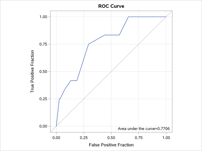
Multinomial-Trial Syntax for Grouped Binary Data
If you have counts of events and nonevents, then instead of using events/trials syntax, you can use the multinomial-trial syntax to perform the same analysis. In the mycas.Ingots data table, the a variable contains the number of ingots ready for rolling (the nonevents). In the following program, you specify the event variable, followed by the nonevent variable:
proc cas;
regression.logistic /
    model={depVars={{name="r"}, {name="a"}},
           effects={{vars={"Heat", "Soak"}},
                    {interaction="CROSS", vars={"Heat", "Soak"}}}},
    table="Ingots";
run;
The only difference from the preceding results is that in this case the "Model Information" table displays the event and nonevent variables; this table is not displayed here.
Single-Trial Syntax for Binary Data
Binomial data are a form of grouped binary data in which "successes" in the underlying Bernoulli trials are totaled. You can thus unwind data for which you use the events/trials syntax and fit these data by using techniques for binary data.
The following DATA step expands the mycas.Ingots data table, which contains 12 events in 387 trials, into a data table that has 387 observations:
proc cas;
dataStep.runCode /
    code="
   data Ingots_binary;
      set Ingots;
      do i=1 to n;
        if i <= r then y=1; else y = 0;
        output;
      end;
   run;
   ",
    single="no";
run;
The following statements fit the model that contains the Heat effect, the Soak effect, and their interaction to the data table. The event=’1’ response-variable subparameter in the model parameter ensures that the logistic action models the probability that the variable y takes the value 1.
proc cas;
regression.logistic /
    model={depVars={{name="y", options={event="1"}}},
           effects={{vars={"Heat", "Soak"}},
                    {interaction="CROSS", vars={"Heat", "Soak"}}}},
    table={name="Ingots_binary"};
run;
Output 22.6.10 displays the "Model Information," "Number of Observations," and "Response Profile" tables. The data are now modeled as binary (Bernoulli distributed) with a logit link function. The "Response Profile" table shows that the binary response breaks down into 375 observations where y=0 and 12 observations where y=1.
Output 22.6.10: Model Information in Binary Model
| Model Information | |
|---|---|
| Data Source | INGOTS_BINARY |
| Response Variable | y |
| Distribution | Binary |
| Link Function | Logit |
| Optimization Technique | Newton-Raphson with Ridging |
Output 22.6.11 displays the result of the test of the global null hypothesis and the parameter estimates. These results match those in Output 22.6.5 and Output 22.6.6.
Output 22.6.11: Null Test and Parameter Estimates
| Testing Global Null Hypothesis: BETA=0 | |||
|---|---|---|---|
| Test | DF | Chi-Square | Pr > ChiSq |
| Likelihood Ratio | 3 | 11.7663 | 0.0082 |
Modeling Binomial Response Data
(View the complete code for this example.)
This section contains Lua code that performs the same analysis as shown in the CASL version of this example.
Note: In order to run this code, the data that are described in the CASL version need to be accessible to the CAS server. One way to do this is to convert the Ingots data to the comma-separated-value (CSV) file Ingots.csv and then use the following code to load the CSV file into CAS:
s:loadtable{casLib="casuser", path="Ingots.csv"}
For more information about coding in Lua, see Getting Started with SAS Viya for Lua and SAS Viya: System Programming Guide.
The following statements use events/trials syntax to model the binomial response. The events variable in this situation is r, and the trials variable is n. The dependency of the probability of not being ready for rolling is modeled as a function of heating time (Heat), soaking time (Soak), and their interaction. The association parameter displays ordinal measures of association between the observed responses and the predicted probabilities. The ctable parameter saves statistics to the Roc data table that are used to evaluate the predictive power of the model. The output parameter stores the linear predictors and the predicted probabilities in the Out data table along with the other variables from the input data table.
s:loadactionset{actionset="regression"}
s:regression.logistic {
   table='Ingots',
   model={depVars={{name='r'}},
          effects={{vars={'Heat', 'Soak'}},
                   {vars={'Heat', 'Soak'}, interaction='CROSS'}},
                    trial='n'},
   output={casOut={name='Out', replace=true},
           copyVars={'Heat', 'Soak'},
           pred='Pred', xBeta='_XBETA_'},
   association=true,
   ctable={casOut={name='Roc', replace=true},
           nocounts=true, tpf='TPF', fpf='FPF'} }
The "Model Information" table shows that the data are modeled as binomially distributed with a logit link function (Output 22.6.12). This is the default link function in the logistic action for binary and binomial data. The action estimates the parameters of the model by a Newton-Raphson algorithm.
Output 22.6.12: Model Information and Number of Observations
| RowId | Description | Value |
|---|---|---|
| DATA | Data Source | INGOTS |
| EVENTVAR | Response Variable (Events) | r |
| TRIALVAR | Response Variable (Trials) | n |
| DIST | Distribution | Binomial |
| LINK | Link Function | Logit |
| TECH | Optimization Technique | Newton-Raphson with Ridging |
| RowId | Description | Value |
|---|---|---|
| NREAD | Number of Observations Read | 19 |
| NUSED | Number of Observations Used | 19 |
| OrderedValue | Outcome | Freq | Modeled |
|---|---|---|---|
| 1 | Event | 12 | * |
| 2 | Nonevent | 375 |
The second table in Output 22.6.12 shows that all 19 observations in the input data table were used in the analysis and the "Response Profile" table shows that the total number of events and nonevents equals 12 and 375, respectively.
Output 22.6.13 displays the convergence status table for this run. The logistic action satisfies the gconv convergence criterion.
Output 22.6.13: Convergence Status
| Reason | Status | MaxGradient | Separation |
|---|---|---|---|
| Convergence criterion (GCONV=1E-8) satisfied. | 0 | 5.42E-11 | 0 |
Output 22.6.14 displays the "Dimensions" table for the model. The design matrix of the model (the matrix) has four columns, which correspond to the intercept, the Heat effect, the Soak effect, and the interaction of the Heat and Soak effects. The model is nonsingular because the rank of the crossproducts matrix equals the number of columns in . All parameters are estimable, and all participate in the optimization.
Output 22.6.14: Dimensions in Binomial Logistic Regression
| RowId | Description | Value |
|---|---|---|
| NDESIGNCOLS | Columns in Design | 4 |
| NEFFECTS | Number of Effects | 4 |
| MAXEFCOLS | Max Effect Columns | 1 |
| DESIGNRANK | Rank of Design | 4 |
| OPTPARM | Parameters in Optimization | 4 |
Output 22.6.15 displays the "Fit Statistics" table for this run. Evaluated at the converged estimates, –2 times the value of the log-likelihood function equals 27.95689. Further fit statistics are also displayed, all of them in "smaller is better" form. The AIC, AICC, and SBC criteria are used to compare non-nested models and to penalize the model fit for the number of observations and parameters. You can use the –2 log-likelihood value to compare nested models by way of a likelihood ratio test.
Output 22.6.15: Fit Statistics
| RowId | Description | Value |
|---|---|---|
| M2LL | -2 Log Likelihood | 27.95689 |
| AIC | AIC (smaller is better) | 35.95689 |
| AICC | AICC (smaller is better) | 38.81403 |
| SBC | SBC (smaller is better) | 39.73464 |
Output 22.6.16 shows the test of the global hypothesis that the effects jointly do not affect the probability of ingot readiness. You can obtain the chi-square test statistic by comparing the –2 log-likelihood value of the model with covariates to the value in the intercept-only model. The test is significant, with a p-value of 0.0082. One or more of the effects in the model have a significant impact on the probability of ingot readiness.
Output 22.6.16: Null Test
| Test | DF | ChiSq | ProbChiSq |
|---|---|---|---|
| Likelihood Ratio | 3 | 11.7663 | 0.0082 |
The "Parameter Estimates" table in Output 22.6.17 displays the estimates and standard errors of the model effects.
Output 22.6.17: Parameter Estimates
| Effect | Parameter | ParmName | DF | Estimate | StdErr | ChiSq | ProbChiSq |
|---|---|---|---|---|---|---|---|
| Intercept | Intercept | Intercept | 1 | -5.990191 | 1.666622 | 12.9183 | 0.0003 |
| Heat | Heat | Heat | 1 | 0.096339 | 0.047067 | 4.1896 | 0.0407 |
| Soak | Soak | Soak | 1 | 0.299574 | 0.755068 | 0.1574 | 0.6916 |
| Heat*Soak | Heat * Soak | Heat___Soak | 1 | -0.008840 | 0.025319 | 0.1219 | 0.7270 |
Output 22.6.18 displays the "Association Statistics" table, which is produced when you specify the association parameter. The table contains four measures of association for assessing the predictive ability of a model. For more information, see the section Association Statistics.
Output 22.6.18: Association of Observed Responses and Predicted Probabilities
| RowId | Description | Value |
|---|---|---|
| C | Concordance Index (AUC) | 0.7706 |
| SOMERSD | Somers' D | 0.5411 |
| GAMMA | Gamma | 0.5858 |
| TAUA | Tau-a | 0.0326 |
| PAIRS | Pairs | 4500 |
| CONCORD | Percent Concordant | 73.2444 |
| DISCORD | Percent Discordant | 19.1333 |
| TIED | Percent Tied | 7.6222 |
You can construct the prediction equation of the model from the "Parameter Estimates" table. For example, an observation with Heat equal to 14 and Soak equal to 1.7 has the linear predictor
The probability that an ingot with these characteristics is not ready for rolling is
The logistic action computes these linear predictors and probabilities and stores them in the Out data table.
The following fetch action from the tables action set enables you to display Output 22.6.19, which shows the probability that an ingot with Heat equal to 14 and Soak equal to 1.7 is not ready for rolling:
s:table_fetch{table={name='Out', where='14 = Heat and 1.7 = Soak'},
              index=false, format=true}
Output 22.6.19: Predicted Probability for Heat=14 and Soak=1.7
| Pred | _XBETA_ | Heat | Soak |
|---|---|---|---|
| 0.0128363197 | -4.34255723 | 14 | 1.7 |
The ctable parameter computes statistics for binary response models (on the basis of classifying observations according to whether their predicted probabilities exceed certain values) and stores the results in the Roc data table. For more information, see the section Classification Table and ROC Curves.
The Roc data table contains information you can use to produce an ROC curve like the following:
Output 22.6.20: Receiver Operating Characteristics Curve
Multinomial-Trial Syntax for Grouped Binary Data
If you have counts of events and nonevents, then instead of using events/trials syntax, you can use the multinomial-trial syntax to perform the same analysis. In the mycas.Ingots data table, the a variable contains the number of ingots ready for rolling (the nonevents). In the following program, you specify the event variable, followed by the nonevent variable:
s:regression.logistic {
   table='Ingots',
   model={depVars={{name='r'},{name='a'}},
          effects={{vars={'Heat', 'Soak'}},
                   {vars={'Heat', 'Soak'}, interaction='CROSS'}}} }
The only difference from the preceding results is that in this case the "Model Information" table displays the event and nonevent variables; this table is not displayed here.
Single-Trial Syntax for Binary Data
Binomial data are a form of grouped binary data in which "successes" in the underlying Bernoulli trials are totaled. You can thus unwind data for which you use the events/trials syntax and fit these data by using techniques for binary data.
The following DATA step expands the Ingots data table, which contains 12 events in 387 trials, into a data table that has 387 observations:
s:dataStep_runCode{single='no', code=[[
data Ingots_binary;
   set Ingots;
   do i=1 to n;
     if i <= r then y=1; else y = 0;
     output;
   end;
run;
]] }
The following statements fit the model that contains the Heat effect, the Soak effect, and their interaction to the data table. The event=’1’ response-variable subparameter in the model parameter ensures that the logistic action models the probability that the variable y takes the value 1.
s:regression_logistic {
   table={name='Ingots_binary'},
   model={depVars={{name='y', options={event='1'}}},
          effects={{vars={'Heat', 'Soak'}},
                   {vars={'Heat', 'Soak'}, interaction='CROSS'}}}}
Output 22.6.21 displays the "Model Information," "Number of Observations," and "Response Profile" tables. The data are now modeled as binary (Bernoulli distributed) with a logit link function. The "Response Profile" table shows that the binary response breaks down into 375 observations where y=0 and 12 observations where y=1.
Output 22.6.21: Model Information in Binary Model
| RowId | Description | Value |
|---|---|---|
| DATA | Data Source | INGOTS_BINARY |
| RESPONSEVAR | Response Variable | y |
| DIST | Distribution | Binary |
| LINK | Link Function | Logit |
| TECH | Optimization Technique | Newton-Raphson with Ridging |
| RowId | Description | Value |
|---|---|---|
| NREAD | Number of Observations Read | 387 |
| NUSED | Number of Observations Used | 387 |
| OrderedValue | Outcome | y | Freq | Modeled |
|---|---|---|---|---|
| 1 | 0 | 0 | 375 | |
| 2 | 1 | 1 | 12 | * |
Output 22.6.22 displays the result of the test of the global null hypothesis and the parameter estimates. These results match those in Output 22.6.16 and Output 22.6.17.
Output 22.6.22: Null Test and Parameter Estimates
| Test | DF | ChiSq | ProbChiSq |
|---|---|---|---|
| Likelihood Ratio | 3 | 11.7663 | 0.0082 |
| Effect | Parameter | ParmName | DF | Estimate | StdErr | ChiSq | ProbChiSq |
|---|---|---|---|---|---|---|---|
| Intercept | Intercept | Intercept | 1 | -5.990191 | 1.666622 | 12.9183 | 0.0003 |
| Heat | Heat | Heat | 1 | 0.096339 | 0.047067 | 4.1896 | 0.0407 |
| Soak | Soak | Soak | 1 | 0.299574 | 0.755068 | 0.1574 | 0.6916 |
| Heat*Soak | Heat * Soak | Heat___Soak | 1 | -0.008840 | 0.025319 | 0.1219 | 0.7270 |
Modeling Binomial Response Data
(View the complete code for this example.)
This section contains Python code that performs the same analysis as shown in the CASL version of this example.
Note: In order to run this code, the data that are described in the CASL version need to be accessible to the CAS server. One way to do this is to convert the Ingots data to the comma-separated-value (CSV) file Ingots.csv and then use the following code to load the CSV file into CAS:
s.upload_file('Ingots.csv')
For more information about coding in Python, see Getting Started with SAS Viya for Python and SAS Viya: System Programming Guide.
The following statements use events/trials syntax to model the binomial response. The events variable in this situation is r, and the trials variable is n. The dependency of the probability of not being ready for rolling is modeled as a function of heating time (Heat), soaking time (Soak), and their interaction. The association parameter displays ordinal measures of association between the observed responses and the predicted probabilities. The ctable parameter saves statistics to the Roc data table that are used to evaluate the predictive power of the model. The output parameter stores the linear predictors and the predicted probabilities in the Out data table along with the other variables from the input data table.
s.loadactionset(actionset='regression')
s.regression.logistic(
    association='true',
    ctable=dict(casOut=dict(name='Roc', replace='true'),
                fpf='FPF',
                nocounts='true',
                tpf='TPF'),
    model=dict(depVars=[dict(name='r')],
               effects=[dict(vars=['Heat', 'Soak']),
                        dict(interaction='CROSS', vars=['Heat', 'Soak'])],
               trial='n'),
    output=dict(casOut=dict(name='Out', replace='true'),
                copyVars=['Heat', 'Soak'],
                pred='Pred',
                xBeta='_XBETA_'),
    table='Ingots')
The "Model Information" table shows that the data are modeled as binomially distributed with a logit link function (Output 22.6.23). This is the default link function in the logistic action for binary and binomial data. The action estimates the parameters of the model by a Newton-Raphson algorithm.
Output 22.6.23: Model Information and Number of Observations
| RowId | Description | Value |
|---|---|---|
| DATA | Data Source | INGOTS |
| EVENTVAR | Response Variable (Events) | r |
| TRIALVAR | Response Variable (Trials) | n |
| DIST | Distribution | Binomial |
| LINK | Link Function | Logit |
| TECH | Optimization Technique | Newton-Raphson with Ridging |
| RowId | Description | Value |
|---|---|---|
| NREAD | Number of Observations Read | 19 |
| NUSED | Number of Observations Used | 19 |
| OrderedValue | Outcome | Freq | Modeled |
|---|---|---|---|
| 1 | Event | 12 | * |
| 2 | Nonevent | 375 |
The second table in Output 22.6.23 shows that all 19 observations in the input data table were used in the analysis and the "Response Profile" table shows that the total number of events and nonevents equals 12 and 375, respectively.
Output 22.6.24 displays the convergence status table for this run. The logistic action satisfies the gconv convergence criterion.
Output 22.6.24: Convergence Status
| Reason | Status | MaxGradient | Separation |
|---|---|---|---|
| Convergence criterion (GCONV=1E-8) satisfied. | 0 | 5.42E-11 | 0 |
Output 22.6.25 displays the "Dimensions" table for the model. The design matrix of the model (the matrix) has four columns, which correspond to the intercept, the Heat effect, the Soak effect, and the interaction of the Heat and Soak effects. The model is nonsingular because the rank of the crossproducts matrix equals the number of columns in . All parameters are estimable, and all participate in the optimization.
Output 22.6.25: Dimensions in Binomial Logistic Regression
| RowId | Description | Value |
|---|---|---|
| NDESIGNCOLS | Columns in Design | 4 |
| NEFFECTS | Number of Effects | 4 |
| MAXEFCOLS | Max Effect Columns | 1 |
| DESIGNRANK | Rank of Design | 4 |
| OPTPARM | Parameters in Optimization | 4 |
Output 22.6.26 displays the "Fit Statistics" table for this run. Evaluated at the converged estimates, –2 times the value of the log-likelihood function equals 27.95689. Further fit statistics are also displayed, all of them in "smaller is better" form. The AIC, AICC, and SBC criteria are used to compare non-nested models and to penalize the model fit for the number of observations and parameters. You can use the –2 log-likelihood value to compare nested models by way of a likelihood ratio test.
Output 22.6.26: Fit Statistics
| RowId | Description | Value |
|---|---|---|
| M2LL | -2 Log Likelihood | 27.95689 |
| AIC | AIC (smaller is better) | 35.95689 |
| AICC | AICC (smaller is better) | 38.81403 |
| SBC | SBC (smaller is better) | 39.73464 |
Output 22.6.27 shows the test of the global hypothesis that the effects jointly do not affect the probability of ingot readiness. You can obtain the chi-square test statistic by comparing the –2 log-likelihood value of the model with covariates to the value in the intercept-only model. The test is significant, with a p-value of 0.0082. One or more of the effects in the model have a significant impact on the probability of ingot readiness.
Output 22.6.27: Null Test
| Test | DF | ChiSq | ProbChiSq |
|---|---|---|---|
| Likelihood Ratio | 3 | 11.7663 | 0.0082 |
The "Parameter Estimates" table in Output 22.6.28 displays the estimates and standard errors of the model effects.
Output 22.6.28: Parameter Estimates
| Effect | Parameter | ParmName | DF | Estimate | StdErr | ChiSq | ProbChiSq |
|---|---|---|---|---|---|---|---|
| Intercept | Intercept | Intercept | 1 | -5.990191 | 1.666622 | 12.9183 | 0.0003 |
| Heat | Heat | Heat | 1 | 0.096339 | 0.047067 | 4.1896 | 0.0407 |
| Soak | Soak | Soak | 1 | 0.299574 | 0.755068 | 0.1574 | 0.6916 |
| Heat*Soak | Heat * Soak | Heat___Soak | 1 | -0.008840 | 0.025319 | 0.1219 | 0.7270 |
Output 22.6.29 displays the "Association Statistics" table, which is produced when you specify the association parameter. The table contains four measures of association for assessing the predictive ability of a model. For more information, see the section Association Statistics.
Output 22.6.29: Association of Observed Responses and Predicted Probabilities
| RowId | Description | Value |
|---|---|---|
| C | Concordance Index (AUC) | 0.7706 |
| SOMERSD | Somers' D | 0.5411 |
| GAMMA | Gamma | 0.5858 |
| TAUA | Tau-a | 0.0326 |
| PAIRS | Pairs | 4500 |
| CONCORD | Percent Concordant | 73.2444 |
| DISCORD | Percent Discordant | 19.1333 |
| TIED | Percent Tied | 7.6222 |
You can construct the prediction equation of the model from the "Parameter Estimates" table. For example, an observation with Heat equal to 14 and Soak equal to 1.7 has the linear predictor
The probability that an ingot with these characteristics is not ready for rolling is
The logistic action computes these linear predictors and probabilities and stores them in the Out data table.
The following fetch action from the tables action set enables you to display Output 22.6.30, which shows the probability that an ingot with Heat equal to 14 and Soak equal to 1.7 is not ready for rolling:
s.table.fetch(
    format='true',
    index='false',
    table=dict(name='Out', where='14 = Heat and 1.7 = Soak'))
Output 22.6.30: Predicted Probability for Heat=14 and Soak=1.7
| Pred | _XBETA_ | Heat | Soak |
|---|---|---|---|
| 0.0128363197 | -4.34255723 | 14 | 1.7 |
The ctable parameter computes statistics for binary response models (on the basis of classifying observations according to whether their predicted probabilities exceed certain values) and stores the results in the Roc data table. For more information, see the section Classification Table and ROC Curves.
The Roc data table contains information you can use to produce an ROC curve like the following:
Output 22.6.31: Receiver Operating Characteristics Curve
Multinomial-Trial Syntax for Grouped Binary Data
If you have counts of events and nonevents, then instead of using events/trials syntax, you can use the multinomial-trial syntax to perform the same analysis. In the mycas.Ingots data table, the a variable contains the number of ingots ready for rolling (the nonevents). In the following program, you specify the event variable, followed by the nonevent variable:
s.regression.logistic(
    model=dict(depVars=[dict(name='r'), dict(name='a')],
               effects=[dict(vars=['Heat', 'Soak']),
                        dict(interaction='CROSS', vars=['Heat', 'Soak'])]),
    table='Ingots')
The only difference from the preceding results is that in this case the "Model Information" table displays the event and nonevent variables; this table is not displayed here.
Single-Trial Syntax for Binary Data
Binomial data are a form of grouped binary data in which "successes" in the underlying Bernoulli trials are totaled. You can thus unwind data for which you use the events/trials syntax and fit these data by using techniques for binary data.
The following DATA step expands the Ingots data table, which contains 12 events in 387 trials, into a data table that has 387 observations:
s.datastep.runcode(
    code='''
   data Ingots_binary;
      set Ingots;
      do i=1 to n;
        if i <= r then y=1; else y = 0;
        output;
      end;
   run;
   ''',
    single='no')
The following statements fit the model that contains the Heat effect, the Soak effect, and their interaction to the data table. The event=’1’ response-variable subparameter in the model parameter ensures that the logistic action models the probability that the variable y takes the value 1.
s.regression.logistic(
    model=dict(depVars=[dict(name='y', options=dict(event='1'))],
               effects=[dict(vars=['Heat', 'Soak']),
                        dict(interaction='CROSS', vars=['Heat', 'Soak'])]),
    table=dict(name='Ingots_binary'))
Output 22.6.32 displays the "Model Information," "Number of Observations," and "Response Profile" tables. The data are now modeled as binary (Bernoulli distributed) with a logit link function. The "Response Profile" table shows that the binary response breaks down into 375 observations where y=0 and 12 observations where y=1.
Output 22.6.32: Model Information in Binary Model
| RowId | Description | Value |
|---|---|---|
| DATA | Data Source | INGOTS_BINARY |
| RESPONSEVAR | Response Variable | y |
| DIST | Distribution | Binary |
| LINK | Link Function | Logit |
| TECH | Optimization Technique | Newton-Raphson with Ridging |
| RowId | Description | Value |
|---|---|---|
| NREAD | Number of Observations Read | 387 |
| NUSED | Number of Observations Used | 387 |
| OrderedValue | Outcome | y | Freq | Modeled |
|---|---|---|---|---|
| 1 | 0 | 0 | 375 | |
| 2 | 1 | 1 | 12 | * |
Output 22.6.33 displays the result of the test of the global null hypothesis and the parameter estimates. These results match those in Output 22.6.27 and Output 22.6.28.
Output 22.6.33: Null Test and Parameter Estimates
| Test | DF | ChiSq | ProbChiSq |
|---|---|---|---|
| Likelihood Ratio | 3 | 11.7663 | 0.0082 |
| Effect | Parameter | ParmName | DF | Estimate | StdErr | ChiSq | ProbChiSq |
|---|---|---|---|---|---|---|---|
| Intercept | Intercept | Intercept | 1 | -5.990191 | 1.666622 | 12.9183 | 0.0003 |
| Heat | Heat | Heat | 1 | 0.096339 | 0.047067 | 4.1896 | 0.0407 |
| Soak | Soak | Soak | 1 | 0.299574 | 0.755068 | 0.1574 | 0.6916 |
| Heat*Soak | Heat * Soak | Heat___Soak | 1 | -0.008840 | 0.025319 | 0.1219 | 0.7270 |
Modeling Binomial Response Data
(View the complete code for this example.)
This section contains R code that performs the same analysis as shown in the CASL version of this example.
Note: In order to run this code, the data that are described in the CASL version need to be accessible to the CAS server. One way to do this is to convert the Ingots data to the comma-separated-value (CSV) file Ingots.csv and then use the following code to load the CSV file into CAS:
m <- cas.read.csv(s, "Ingots.csv", casOut=list(name="Ingots"))
For more information about coding in R, see Getting Started with SAS Viya for R and SAS Viya: System Programming Guide.
The following statements use events/trials syntax to model the binomial response. The events variable in this situation is r, and the trials variable is n. The dependency of the probability of not being ready for rolling is modeled as a function of heating time (Heat), soaking time (Soak), and their interaction. The association parameter displays ordinal measures of association between the observed responses and the predicted probabilities. The ctable parameter saves statistics to the Roc data table that are used to evaluate the predictive power of the model. The output parameter stores the linear predictors and the predicted probabilities in the Out data table along with the other variables from the input data table.
m <- cas.builtins.loadActionSet(s, actionset='regression')
cas.regression.logistic(s,
    association='true',
    ctable=list(casOut=list(name='Roc', replace='true'),
                fpf='FPF',
                nocounts='true',
                tpf='TPF'),
    model=list(depVars=list(list(name='r')),
               effects=list(list(vars=c('Heat', 'Soak')),
                            list(interaction='CROSS', vars=c('Heat', 'Soak'))),
               trial='n'),
    output=list(casOut=list(name='Out', replace='true'),
                copyVars=c('Heat', 'Soak'),
                pred='Pred',
                xBeta='_XBETA_'),
    table='Ingots')
The "Model Information" table shows that the data are modeled as binomially distributed with a logit link function (Output 22.6.34). This is the default link function in the logistic action for binary and binomial data. The action estimates the parameters of the model by a Newton-Raphson algorithm.
Output 22.6.34: Model Information and Number of Observations
| RowId | Description | Value |
|---|---|---|
| DATA | Data Source | INGOTS |
| EVENTVAR | Response Variable (Events) | r |
| TRIALVAR | Response Variable (Trials) | n |
| DIST | Distribution | Binomial |
| LINK | Link Function | Logit |
| TECH | Optimization Technique | Newton-Raphson with Ridging |
| RowId | Description | Value |
|---|---|---|
| NREAD | Number of Observations Read | 19 |
| NUSED | Number of Observations Used | 19 |
| OrderedValue | Outcome | Freq | Modeled |
|---|---|---|---|
| 1 | Event | 12 | * |
| 2 | Nonevent | 375 |
The second table in Output 22.6.34 shows that all 19 observations in the input data table were used in the analysis and the "Response Profile" table shows that the total number of events and nonevents equals 12 and 375, respectively.
Output 22.6.35 displays the convergence status table for this run. The logistic action satisfies the gconv convergence criterion.
Output 22.6.35: Convergence Status
| Reason | Status | MaxGradient | Separation |
|---|---|---|---|
| Convergence criterion (GCONV=1E-8) satisfied. | 0 | 5.42E-11 | 0 |
Output 22.6.36 displays the "Dimensions" table for the model. The design matrix of the model (the matrix) has four columns, which correspond to the intercept, the Heat effect, the Soak effect, and the interaction of the Heat and Soak effects. The model is nonsingular because the rank of the crossproducts matrix equals the number of columns in . All parameters are estimable, and all participate in the optimization.
Output 22.6.36: Dimensions in Binomial Logistic Regression
| RowId | Description | Value |
|---|---|---|
| NDESIGNCOLS | Columns in Design | 4 |
| NEFFECTS | Number of Effects | 4 |
| MAXEFCOLS | Max Effect Columns | 1 |
| DESIGNRANK | Rank of Design | 4 |
| OPTPARM | Parameters in Optimization | 4 |
Output 22.6.37 displays the "Fit Statistics" table for this run. Evaluated at the converged estimates, –2 times the value of the log-likelihood function equals 27.95689. Further fit statistics are also displayed, all of them in "smaller is better" form. The AIC, AICC, and SBC criteria are used to compare non-nested models and to penalize the model fit for the number of observations and parameters. You can use the –2 log-likelihood value to compare nested models by way of a likelihood ratio test.
Output 22.6.37: Fit Statistics
| RowId | Description | Value |
|---|---|---|
| M2LL | -2 Log Likelihood | 27.95689 |
| AIC | AIC (smaller is better) | 35.95689 |
| AICC | AICC (smaller is better) | 38.81403 |
| SBC | SBC (smaller is better) | 39.73464 |
Output 22.6.38 shows the test of the global hypothesis that the effects jointly do not affect the probability of ingot readiness. You can obtain the chi-square test statistic by comparing the –2 log-likelihood value of the model with covariates to the value in the intercept-only model. The test is significant, with a p-value of 0.0082. One or more of the effects in the model have a significant impact on the probability of ingot readiness.
Output 22.6.38: Null Test
| Test | DF | ChiSq | ProbChiSq |
|---|---|---|---|
| Likelihood Ratio | 3 | 11.7663 | 0.0082 |
The "Parameter Estimates" table in Output 22.6.39 displays the estimates and standard errors of the model effects.
Output 22.6.39: Parameter Estimates
| Effect | Parameter | ParmName | DF | Estimate | StdErr | ChiSq | ProbChiSq |
|---|---|---|---|---|---|---|---|
| Intercept | Intercept | Intercept | 1 | -5.990191 | 1.666622 | 12.9183 | 0.0003 |
| Heat | Heat | Heat | 1 | 0.096339 | 0.047067 | 4.1896 | 0.0407 |
| Soak | Soak | Soak | 1 | 0.299574 | 0.755068 | 0.1574 | 0.6916 |
| Heat*Soak | Heat * Soak | Heat___Soak | 1 | -0.008840 | 0.025319 | 0.1219 | 0.7270 |
Output 22.6.40 displays the "Association Statistics" table, which is produced when you specify the association parameter. The table contains four measures of association for assessing the predictive ability of a model. For more information, see the section Association Statistics.
Output 22.6.40: Association of Observed Responses and Predicted Probabilities
| RowId | Description | Value |
|---|---|---|
| C | Concordance Index (AUC) | 0.7706 |
| SOMERSD | Somers' D | 0.5411 |
| GAMMA | Gamma | 0.5858 |
| TAUA | Tau-a | 0.0326 |
| PAIRS | Pairs | 4500 |
| CONCORD | Percent Concordant | 73.2444 |
| DISCORD | Percent Discordant | 19.1333 |
| TIED | Percent Tied | 7.6222 |
You can construct the prediction equation of the model from the "Parameter Estimates" table. For example, an observation with Heat equal to 14 and Soak equal to 1.7 has the linear predictor
The probability that an ingot with these characteristics is not ready for rolling is
The logistic action computes these linear predictors and probabilities and stores them in the Out data table.
The following fetch action from the tables action set enables you to display Output 22.6.41, which shows the probability that an ingot with Heat equal to 14 and Soak equal to 1.7 is not ready for rolling:
cas.table.fetch(s,
    format='true',
    index='false',
    table=list(name='Out', where='14 = Heat and 1.7 = Soak'))
Output 22.6.41: Predicted Probability for Heat=14 and Soak=1.7
| Pred | _XBETA_ | Heat | Soak |
|---|---|---|---|
| 0.0128363197 | -4.34255723 | 14 | 1.7 |
The ctable parameter computes statistics for binary response models (on the basis of classifying observations according to whether their predicted probabilities exceed certain values) and stores the results in the Roc data table. For more information, see the section Classification Table and ROC Curves.
The Roc data table contains information you can use to produce an ROC curve like the following:
Output 22.6.42: Receiver Operating Characteristics Curve
Multinomial-Trial Syntax for Grouped Binary Data
If you have counts of events and nonevents, then instead of using events/trials syntax, you can use the multinomial-trial syntax to perform the same analysis. In the mycas.Ingots data table, the a variable contains the number of ingots ready for rolling (the nonevents). In the following program, you specify the event variable, followed by the nonevent variable:
cas.regression.logistic(s,
    model=list(depVars=list(list(name='r'), list(name='a')),
               effects=list(list(vars=c('Heat', 'Soak')),
                            list(interaction='CROSS', vars=c('Heat', 'Soak')))),
    table='Ingots')
The only difference from the preceding results is that in this case the "Model Information" table displays the event and nonevent variables; this table is not displayed here.
Single-Trial Syntax for Binary Data
Binomial data are a form of grouped binary data in which "successes" in the underlying Bernoulli trials are totaled. You can thus unwind data for which you use the events/trials syntax and fit these data by using techniques for binary data.
The following DATA step expands the Ingots data table, which contains 12 events in 387 trials, into a data table that has 387 observations:
cas.dataStep.runCode(s,
    code='
   data Ingots_binary;
      set Ingots;
      do i=1 to n;
        if i <= r then y=1; else y = 0;
        output;
      end;
   run;
   ',
    single='no')
The following statements fit the model that contains the Heat effect, the Soak effect, and their interaction to the data table. The event=’1’ response-variable subparameter in the model parameter ensures that the logistic action models the probability that the variable y takes the value 1.
cas.regression.logistic(s,
    model=list(depVars=list(list(name='y', options=list(event='1'))),
               effects=list(list(vars=c('Heat', 'Soak')),
                            list(interaction='CROSS', vars=c('Heat', 'Soak')))),
    table=list(name='Ingots_binary'))
Output 22.6.43 displays the "Model Information," "Number of Observations," and "Response Profile" tables. The data are now modeled as binary (Bernoulli distributed) with a logit link function. The "Response Profile" table shows that the binary response breaks down into 375 observations where y=0 and 12 observations where y=1.
Output 22.6.43: Model Information in Binary Model
| RowId | Description | Value |
|---|---|---|
| DATA | Data Source | INGOTS_BINARY |
| RESPONSEVAR | Response Variable | y |
| DIST | Distribution | Binary |
| LINK | Link Function | Logit |
| TECH | Optimization Technique | Newton-Raphson with Ridging |
| RowId | Description | Value |
|---|---|---|
| NREAD | Number of Observations Read | 387 |
| NUSED | Number of Observations Used | 387 |
| OrderedValue | Outcome | y | Freq | Modeled |
|---|---|---|---|---|
| 1 | 0 | 0 | 375 | |
| 2 | 1 | 1 | 12 | * |
Output 22.6.44 displays the result of the test of the global null hypothesis and the parameter estimates. These results match those in Output 22.6.38 and Output 22.6.39.
Output 22.6.44: Null Test and Parameter Estimates
| Test | DF | ChiSq | ProbChiSq |
|---|---|---|---|
| Likelihood Ratio | 3 | 11.7663 | 0.0082 |
| Effect | Parameter | ParmName | DF | Estimate | StdErr | ChiSq | ProbChiSq |
|---|---|---|---|---|---|---|---|
| Intercept | Intercept | Intercept | 1 | -5.990191 | 1.666622 | 12.9183 | 0.0003 |
| Heat | Heat | Heat | 1 | 0.096339 | 0.047067 | 4.1896 | 0.0407 |
| Soak | Soak | Soak | 1 | 0.299574 | 0.755068 | 0.1574 | 0.6916 |
| Heat*Soak | Heat * Soak | Heat___Soak | 1 | -0.008840 | 0.025319 | 0.1219 | 0.7270 |
Computing Odds Ratios
(View the complete code for this example.)
This section uses the data and selected model from Example 22.5 to demonstrate how to request odds ratios. In the following statements, the oddsratio parameter is specified to compute the odds ratios, and the variables for which odds ratios are computed are listed in the vars subparameter.
proc cas;
regression.logistic /
    display="oddsratios",
    model={depvar={{name="y", options={event="1"}}}, effects={"x2", "x8"}},
    oddsratios={vars={"x2", "x8"}},
    table="getStarted";
run;
The resulting odds ratios are displayed in Output 22.7.1.
Output 22.7.1: Odds Ratios for Main Effects
| Odds Ratios | |||||
|---|---|---|---|---|---|
| Description | Estimate | 95% Wald Confidence Limits |
p-Value | Percent Change |
|
| x2 | 3.163 | 2.041 | 4.902 | <.0001 | 216.26 |
| x8 | 2.804 | 1.790 | 4.391 | <.0001 | 180.36 |
From Output 22.7.1, subjects with an X2 value that is one unit larger than its current value have 3.163 times the odds of having a Y = 1 response, and subjects with an X8 value that is one unit larger have 2.804 times the odds.
If your model has interactions, then the odds ratio computations depend on the values of the interacting variables. The following code produces odds ratios for the main effects, but because of interactions, these odds ratios depend on the values of the interacting variables as displayed in Output 22.7.2:
proc cas;
regression.logistic /
    display="oddsratios",
    model={depvar={{name="y", options={event="1"}}},
           effects={{interaction="BAR", vars={"x2", "x8"}}}},
    oddsratios={vars={"x2", "x8"}},
    table="getStarted";
run;
Output 22.7.2: Default Odds Ratios with Interactions
| Odds Ratios | |||||
|---|---|---|---|---|---|
| Description | Estimate | 95% Wald Confidence Limits |
p-Value | Percent Change |
|
| x2 at x8=0.0087 | 2.379 | 1.014 | 5.582 | 0.0464 | 137.89 |
| x8 at x2=0.0101429 | 2.143 | 0.941 | 4.882 | 0.0695 | 114.35 |
The odds ratios in Output 22.7.2 are computed at the mean values of the interacting variables. You can change these values by specifying an at parameter for each individual odds ratio, as follows:
proc cas;
regression.logistic /
    display="oddsratios",
    model={depvar={{name="y", options={event="1"}}},
           effects={{interaction="BAR", vars={"x2", "x8"}}}},
    oddsratios={vars={{at={{value="2", var="x8"}}, var="x2"},
                      {at={{value={5, 10}, var="x2"}}, var="x8"}}},
    table="getStarted";
run;
Output 22.7.3: Customized Odds Ratios
| Odds Ratios | |||||
|---|---|---|---|---|---|
| Description | Estimate | 95% Wald Confidence Limits |
p-Value | Percent Change |
|
| x2 at x8=2 | 7.684 | 0.743 | 79.435 | 0.0871 | 668.36 |
| x8 at x2=5 | 40.463 | 0.040 | >999.999 | 0.2937 | 3946.33 |
| x8 at x2=10 | 768.416 | <0.001 | >999.999 | 0.3691 | 76741.57 |
The following commands customize these odds ratios by using individual options to compute the change in the odds when X2 is increased by 5 and 10 units, and by considering only levels of C equal to "A" or "B" and setting X8 to 1. The results are displayed in Output 22.7.4.
proc cas;
regression.logistic /
    class={"C"},
    display="oddsratios",
    model={depvar={{name="y", options={event="1"}}},
           effects={{interaction="BAR", vars={"C", "x2", "x8"}}}},
    oddsratios={vars={{at={{level={"A", "B"}, var="C"}, {values={1}, var="x8"}},
                       unit={5, 10},
                       var="x2"}}},
    table="getStarted";
run;
Output 22.7.4: Customized Odds Ratios
| Odds Ratios | |||||
|---|---|---|---|---|---|
| Description | Estimate | 95% Wald Confidence Limits |
p-Value | Percent Change |
|
| x2 units=5 at C=A x8=1 | 73.319 | <0.001 | >999.999 | 0.5669 | 7231.87 |
| x2 units=5 at C=B x8=1 | >999.999 | 0.049 | >999.999 | 0.1186 | 13364538 |
| x2 units=10 at C=A x8=1 | >999.999 | <0.001 | >999.999 | 0.5669 | 537463.3 |
| x2 units=10 at C=B x8=1 | >999.999 | 0.002 | >999.999 | 0.1186 | 1.786E12 |
You can perform the same customization by specifying global options as follows:
proc cas;
regression.logistic /
    class={"C"},
    display="oddsratios",
    model={depvar={{name="y", options={event="1"}}},
           effects={{interaction="BAR", vars={"C", "x2", "x8"}}}},
    oddsratios={at={{level={"A", "B"}, var="C"}, {values={1}, var="x8"}},
                unit={{value={5, 10}, var="x2"}},
                vars="x2"},
    table="getStarted";
run;
Computing Odds Ratios
(View the complete code for this example.)
This section uses the data and selected model from Example 22.5 to demonstrate how to request odds ratios. In the following statements, the oddsratio parameter is specified to compute the odds ratios, and the variables for which odds ratios are computed are listed in the vars subparameter.
s:regression_logistic{
   table='getStarted',
   model={depvar={{name='y', options={event='1'}}},
          effects={'x2', 'x8'}},
   oddsratios={vars={'x2', 'x8'}},
   display='oddsratios' }
The resulting odds ratios are displayed in Output 22.7.5.
Output 22.7.5: Odds Ratios for Main Effects
| Description | Estimate | Alpha | LowerWaldCL | UpperWaldCL | WaldPValue | PctChangeInOdds | Variable |
|---|---|---|---|---|---|---|---|
| x2 | 3.163 | 0.05 | 2.041 | 4.902 | <.0001 | 216.26 | x2 |
| x8 | 2.804 | 0.05 | 1.790 | 4.391 | <.0001 | 180.36 | x8 |
From Output 22.7.5, subjects with an X2 value that is one unit larger than its current value have 3.163 times the odds of having a Y = 1 response, and subjects with an X8 value that is one unit larger have 2.804 times the odds.
If your model has interactions, then the odds ratio computations depend on the values of the interacting variables. The following code produces odds ratios for the main effects, but because of interactions, these odds ratios depend on the values of the interacting variables as displayed in Output 22.7.6:
s:regression_logistic{
   table='getStarted',
   model={depvar={{name='y', options={event='1'}}},
          effects={{vars={'x2', 'x8'},interaction='BAR'}}},
   oddsratios={vars={'x2','x8'}},
   display='oddsratios' }
Output 22.7.6: Default Odds Ratios with Interactions
| Description | Estimate | Alpha | LowerWaldCL | UpperWaldCL | WaldPValue | PctChangeInOdds | Variable | At |
|---|---|---|---|---|---|---|---|---|
| x2 at x8=0.0087 | 2.379 | 0.05 | 1.014 | 5.582 | 0.0464 | 137.89 | x2 | x8=0.0087 |
| x8 at x2=0.0101429 | 2.143 | 0.05 | 0.941 | 4.882 | 0.0695 | 114.35 | x8 | x2=0.0101429 |
The odds ratios in Output 22.7.6 are computed at the mean values of the interacting variables. You can change these values by specifying an at parameter for each individual odds ratio, as follows:
s:regression_logistic{
   table='getStarted',
   model={depvar={{name='y', options={event='1'}}},
          effects={{vars={'x2', 'x8'},interaction='BAR'}}},
   oddsratios={vars={{var='x2',at={{var='x8',value=2}}},
                     {var='x8',at={{var='x2',value={5,10}}}}}},
   display='oddsratios' }
Output 22.7.7: Customized Odds Ratios
| Description | Estimate | Alpha | LowerWaldCL | UpperWaldCL | WaldPValue | PctChangeInOdds | Variable | At |
|---|---|---|---|---|---|---|---|---|
| x2 at x8=2 | 7.684 | 0.05 | 0.743 | 79.435 | 0.0871 | 668.36 | x2 | x8=2 |
| x8 at x2=5 | 40.463 | 0.05 | 0.040 | >999.999 | 0.2937 | 3946.33 | x8 | x2=5 |
| x8 at x2=10 | 768.416 | 0.05 | <0.001 | >999.999 | 0.3691 | 76741.57 | x8 | x2=10 |
The following commands customize these odds ratios by using individual options to compute the change in the odds when X2 is increased by 5 and 10 units, and by considering only levels of C equal to "A" or "B" and setting X8 to 1. The results are displayed in Output 22.7.8.
s:regression_logistic{
   table='getStarted',
   class={'C'},
   model={depvar={{name='y', options={event='1'}}},
          effects={{vars={'C', 'x2', 'x8'}, interaction='BAR'}}},
   oddsratios={vars={
      {var='x2',unit={5,10},at={{var='C',level={'A','B'}},
                                {var='x8',values={1}} } } }},
   display='oddsratios' }
Output 22.7.8: Customized Odds Ratios
| Description | Estimate | Alpha | LowerWaldCL | UpperWaldCL | WaldPValue | PctChangeInOdds | Variable | Units | At |
|---|---|---|---|---|---|---|---|---|---|
| x2 units=5 at C=A x8=1 | 73.319 | 0.05 | <0.001 | >999.999 | 0.5669 | 7231.87 | x2 | 5 | C=A x8=1 |
| x2 units=5 at C=B x8=1 | >999.999 | 0.05 | 0.049 | >999.999 | 0.1186 | 13364538 | x2 | 5 | C=B x8=1 |
| x2 units=10 at C=A x8=1 | >999.999 | 0.05 | <0.001 | >999.999 | 0.5669 | 537463.3 | x2 | 10 | C=A x8=1 |
| x2 units=10 at C=B x8=1 | >999.999 | 0.05 | 0.002 | >999.999 | 0.1186 | 1.786E12 | x2 | 10 | C=B x8=1 |
You can perform the same customization by specifying global options as follows:
s:regression_logistic{
   table='getStarted',
   class={'C'},
   model={depvar={{name='y', options={event='1'}}},
          effects={{vars={'C', 'x2', 'x8'},interaction='BAR'}}},
   oddsratios={vars='x2',
               unit={{var='x2',value={5,10}}},
               at={{var='C',level={'A','B'}},
                   {var='x8',values={1}} }},
   display='oddsratios' }
Computing Odds Ratios
(View the complete code for this example.)
This section uses the data and selected model from Example 22.5 to demonstrate how to request odds ratios. In the following statements, the oddsratio parameter is specified to compute the odds ratios, and the variables for which odds ratios are computed are listed in the vars subparameter.
s.regression.logistic(
    display='oddsratios',
    model=dict(depvar=[dict(name='y', options=dict(event='1'))],
               effects=['x2', 'x8']),
    oddsratios=dict(vars=['x2', 'x8']),
    table='getStarted')
The resulting odds ratios are displayed in Output 22.7.9.
Output 22.7.9: Odds Ratios for Main Effects
| Description | Estimate | Alpha | LowerWaldCL | UpperWaldCL | WaldPValue | PctChangeInOdds | Variable |
|---|---|---|---|---|---|---|---|
| x2 | 3.163 | 0.05 | 2.041 | 4.902 | <.0001 | 216.26 | x2 |
| x8 | 2.804 | 0.05 | 1.790 | 4.391 | <.0001 | 180.36 | x8 |
From Output 22.7.9, subjects with an X2 value that is one unit larger than its current value have 3.163 times the odds of having a Y = 1 response, and subjects with an X8 value that is one unit larger have 2.804 times the odds.
If your model has interactions, then the odds ratio computations depend on the values of the interacting variables. The following code produces odds ratios for the main effects, but because of interactions, these odds ratios depend on the values of the interacting variables as displayed in Output 22.7.10:
s.regression.logistic(
    display='oddsratios',
    model=dict(depvar=[dict(name='y', options=dict(event='1'))],
               effects=[dict(interaction='BAR', vars=['x2', 'x8'])]),
    oddsratios=dict(vars=['x2', 'x8']),
    table='getStarted')
Output 22.7.10: Default Odds Ratios with Interactions
| Description | Estimate | Alpha | LowerWaldCL | UpperWaldCL | WaldPValue | PctChangeInOdds | Variable | At |
|---|---|---|---|---|---|---|---|---|
| x2 at x8=0.0087 | 2.379 | 0.05 | 1.014 | 5.582 | 0.0464 | 137.89 | x2 | x8=0.0087 |
| x8 at x2=0.0101429 | 2.143 | 0.05 | 0.941 | 4.882 | 0.0695 | 114.35 | x8 | x2=0.0101429 |
The odds ratios in Output 22.7.10 are computed at the mean values of the interacting variables. You can change these values by specifying an at parameter for each individual odds ratio, as follows:
s.regression.logistic(
    display='oddsratios',
    model=dict(depvar=[dict(name='y', options=dict(event='1'))],
               effects=[dict(interaction='BAR', vars=['x2', 'x8'])]),
    oddsratios=dict(vars=[dict(at=[dict(value='2', var='x8')], var='x2'),
                          dict(at=[dict(value=[5, 10], var='x2')], var='x8')]),
    table='getStarted')
Output 22.7.11: Customized Odds Ratios
| Description | Estimate | Alpha | LowerWaldCL | UpperWaldCL | WaldPValue | PctChangeInOdds | Variable | At |
|---|---|---|---|---|---|---|---|---|
| x2 at x8=2 | 7.684 | 0.05 | 0.743 | 79.435 | 0.0871 | 668.36 | x2 | x8=2 |
| x8 at x2=5 | 40.463 | 0.05 | 0.040 | >999.999 | 0.2937 | 3946.33 | x8 | x2=5 |
| x8 at x2=10 | 768.416 | 0.05 | <0.001 | >999.999 | 0.3691 | 76741.57 | x8 | x2=10 |
The following commands customize these odds ratios by using individual options to compute the change in the odds when X2 is increased by 5 and 10 units, and by considering only levels of C equal to "A" or "B" and setting X8 to 1. The results are displayed in Output 22.7.12.
s.regression.logistic(
    class_=['C'],
    display='oddsratios',
    model=dict(depvar=[dict(name='y', options=dict(event='1'))],
               effects=[dict(interaction='BAR', vars=['C', 'x2', 'x8'])]),
    oddsratios=dict(vars=[dict(at=[dict(level=['A', 'B'], var='C'),
                                   dict(values=[1], var='x8')],
                               unit=[5, 10],
                               var='x2')]),
    table='getStarted')
Output 22.7.12: Customized Odds Ratios
| Description | Estimate | Alpha | LowerWaldCL | UpperWaldCL | WaldPValue | PctChangeInOdds | Variable | Units | At |
|---|---|---|---|---|---|---|---|---|---|
| x2 units=5 at C=A x8=1 | 73.319 | 0.05 | <0.001 | >999.999 | 0.5669 | 7231.87 | x2 | 5 | C=A x8=1 |
| x2 units=5 at C=B x8=1 | >999.999 | 0.05 | 0.049 | >999.999 | 0.1186 | 13364538 | x2 | 5 | C=B x8=1 |
| x2 units=10 at C=A x8=1 | >999.999 | 0.05 | <0.001 | >999.999 | 0.5669 | 537463.3 | x2 | 10 | C=A x8=1 |
| x2 units=10 at C=B x8=1 | >999.999 | 0.05 | 0.002 | >999.999 | 0.1186 | 1.786E12 | x2 | 10 | C=B x8=1 |
You can perform the same customization by specifying global options as follows:
s.regression.logistic(
    class_=['C'],
    display='oddsratios',
    model=dict(depvar=[dict(name='y', options=dict(event='1'))],
               effects=[dict(interaction='BAR', vars=['C', 'x2', 'x8'])]),
    oddsratios=dict(at=[dict(level=['A', 'B'], var='C'),
                        dict(values=[1], var='x8')],
                    unit=[dict(value=[5, 10], var='x2')],
                    vars='x2'),
    table='getStarted')
Computing Odds Ratios
(View the complete code for this example.)
This section uses the data and selected model from Example 22.5 to demonstrate how to request odds ratios. In the following statements, the oddsratio parameter is specified to compute the odds ratios, and the variables for which odds ratios are computed are listed in the vars subparameter.
cas.regression.logistic(s,
    display='oddsratios',
    model=list(depvar=list(list(name='y', options=list(event='1'))),
               effects=c('x2', 'x8')),
    oddsratios=list(vars=c('x2', 'x8')),
    table='getStarted')
The resulting odds ratios are displayed in Output 22.7.13.
Output 22.7.13: Odds Ratios for Main Effects
| Description | Estimate | Alpha | LowerWaldCL | UpperWaldCL | WaldPValue | PctChangeInOdds | Variable |
|---|---|---|---|---|---|---|---|
| x2 | 3.163 | 0.05 | 2.041 | 4.902 | <.0001 | 216.26 | x2 |
| x8 | 2.804 | 0.05 | 1.790 | 4.391 | <.0001 | 180.36 | x8 |
From Output 22.7.13, subjects with an X2 value that is one unit larger than its current value have 3.163 times the odds of having a Y = 1 response, and subjects with an X8 value that is one unit larger have 2.804 times the odds.
If your model has interactions, then the odds ratio computations depend on the values of the interacting variables. The following code produces odds ratios for the main effects, but because of interactions, these odds ratios depend on the values of the interacting variables as displayed in Output 22.7.14:
cas.regression.logistic(s,
    display='oddsratios',
    model=list(depvar=list(list(name='y', options=list(event='1'))),
               effects=list(list(interaction='BAR', vars=c('x2', 'x8')))),
    oddsratios=list(vars=c('x2', 'x8')),
    table='getStarted')
Output 22.7.14: Default Odds Ratios with Interactions
| Description | Estimate | Alpha | LowerWaldCL | UpperWaldCL | WaldPValue | PctChangeInOdds | Variable | At |
|---|---|---|---|---|---|---|---|---|
| x2 at x8=0.0087 | 2.379 | 0.05 | 1.014 | 5.582 | 0.0464 | 137.89 | x2 | x8=0.0087 |
| x8 at x2=0.0101429 | 2.143 | 0.05 | 0.941 | 4.882 | 0.0695 | 114.35 | x8 | x2=0.0101429 |
The odds ratios in Output 22.7.14 are computed at the mean values of the interacting variables. You can change these values by specifying an at parameter for each individual odds ratio, as follows:
cas.regression.logistic(s,
    display='oddsratios',
    model=list(depvar=list(list(name='y', options=list(event='1'))),
               effects=list(list(interaction='BAR', vars=c('x2', 'x8')))),
    oddsratios=list(vars=list(list(at=list(list(value='2', var='x8')),
                                   var='x2'),
                              list(at=list(list(value=c(5, 10), var='x2')),
                                   var='x8'))),
    table='getStarted')
Output 22.7.15: Customized Odds Ratios
| Description | Estimate | Alpha | LowerWaldCL | UpperWaldCL | WaldPValue | PctChangeInOdds | Variable | At |
|---|---|---|---|---|---|---|---|---|
| x2 at x8=2 | 7.684 | 0.05 | 0.743 | 79.435 | 0.0871 | 668.36 | x2 | x8=2 |
| x8 at x2=5 | 40.463 | 0.05 | 0.040 | >999.999 | 0.2937 | 3946.33 | x8 | x2=5 |
| x8 at x2=10 | 768.416 | 0.05 | <0.001 | >999.999 | 0.3691 | 76741.57 | x8 | x2=10 |
The following commands customize these odds ratios by using individual options to compute the change in the odds when X2 is increased by 5 and 10 units, and by considering only levels of C equal to "A" or "B" and setting X8 to 1. The results are displayed in Output 22.7.16.
cas.regression.logistic(s,
    class=c('C'),
    display='oddsratios',
    model=list(depvar=list(list(name='y', options=list(event='1'))),
               effects=list(list(interaction='BAR', vars=c('C', 'x2', 'x8')))),
    oddsratios=list(vars=list(list(at=list(list(level=c('A', 'B'), var='C'),
                                           list(values=c(1), var='x8')),
                                   unit=c(5, 10),
                                   var='x2'))),
    table='getStarted')
Output 22.7.16: Customized Odds Ratios
| Description | Estimate | Alpha | LowerWaldCL | UpperWaldCL | WaldPValue | PctChangeInOdds | Variable | Units | At |
|---|---|---|---|---|---|---|---|---|---|
| x2 units=5 at C=A x8=1 | 73.319 | 0.05 | <0.001 | >999.999 | 0.5669 | 7231.87 | x2 | 5 | C=A x8=1 |
| x2 units=5 at C=B x8=1 | >999.999 | 0.05 | 0.049 | >999.999 | 0.1186 | 13364538 | x2 | 5 | C=B x8=1 |
| x2 units=10 at C=A x8=1 | >999.999 | 0.05 | <0.001 | >999.999 | 0.5669 | 537463.3 | x2 | 10 | C=A x8=1 |
| x2 units=10 at C=B x8=1 | >999.999 | 0.05 | 0.002 | >999.999 | 0.1186 | 1.786E12 | x2 | 10 | C=B x8=1 |
You can perform the same customization by specifying global options as follows:
cas.regression.logistic(s,
    class=c('C'),
    display='oddsratios',
    model=list(depvar=list(list(name='y', options=list(event='1'))),
               effects=list(list(interaction='BAR', vars=c('C', 'x2', 'x8')))),
    oddsratios=list(at=list(list(level=c('A', 'B'), var='C'),
                            list(values=c(1), var='x8')),
                    unit=list(list(value=c(5, 10), var='x2')),
                    vars='x2'),
    table='getStarted')