UCM Procedure
Example 41.10 A Transfer-Function Model for the Italian Traffic Accident Data
(View the complete code for this example.)
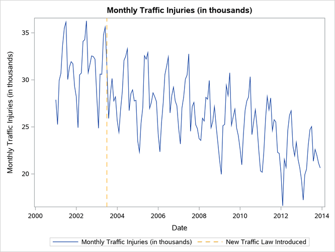
This example is based on a case study described in Pelagatti (2015, chap. 9, sec. 1). In July 2003, Italy introduced a new traffic monitoring system with the aim of improving traffic safety. The case study tried to answer the question, "Was the monitoring system effective in reducing the number of traffic injuries?" The time series plot in Output 41.10.1 shows monthly traffic injuries for the span of January 2001 to December 2013. Visual inspection of the plot clearly shows that the series is seasonal and has an overall downward trend, which appears to be more pronounced after the intervention.
Output 41.10.1: Monthly Traffic Injuries in Italy
Pelagatti (2015, chap. 9, sec. 1) suggests the following model for this series:

Various terms in the right-hand side of this model are explained as follows:
 is the trend component, which is modeled as an integrated random walk.
  is the trigonometric seasonal component, which accounts for the monthly seasonality.
 -
The effect of the introduction of the monitoring system is modeled using two terms:
One term captures a permanent shift, which is a regression effect that is associated with the dummy regressor
shift03. This regressor is 0 before July 2003 and 1 thereafter.-
The other term captures a transient effect that rapidly decays to 0. The transient effect
 is a transfer-function effect
where
pulse03is a dummy regressor that is 1 at July 2003 and 0 otherwise. In this example, the transfer function is clearly 0 before July 2003.
 is the simple irregular component.
The following statements show how to fit this model to the data. The LIKE=MARGINAL option in the ESTIMATE statement causes the parameter estimation to be based on marginal likelihood rather than on diffuse likelihood, which is the default. Since the parameter vector of this model contains  (the denominator coefficient of the transfer function), the parameter estimations that are based on marginal likelihood and diffuse likelihood can lead to different results. In this example, the results turn out to be similar; however, this is not necessarily the case in general. Generally, parameter estimation that is based on marginal likelihood is the preferred choice in such cases.
proc ucm data=italy;
   id date interval=month;
   model Injured = shift03;
   irregular;
   level variance=0 noest;
   slope;
   season length=12 type=trig;
   tf pulse03 den=1 tfstart=0 plot=smooth;
   estimate plot=(panel residual) like=marginal;
   forecast plot=decomp;
run;
Output 41.10.3 shows the parameter estimates. It shows that soon after the introduction of the monitoring system in July 2003, the accident level decreased by about 5.22 thousand ( ). However, the permanent decrease was only about 2.48 thousand (
 ). The estimate of the decay parameter of the transfer function, , is 0.587.
Output 41.10.2: Estimates of the Model Parameters
| Final Estimates of the Free Parameters | |||||
|---|---|---|---|---|---|
| Component | Parameter | Estimate | Approx Std Error |
t Value | Approx Pr > |t| |
| Irregular | Error Variance | 0.55447 | 0.09227 | 6.01 | <.0001 |
| Slope | Error Variance | 0.00064586 | 0.0004515 | 1.43 | 0.1526 |
| Season | Error Variance | 0.00068803 | 0.0005190 | 1.33 | 0.1849 |
| shift03 | Coefficient | -2.47939 | 0.70928 | -3.50 | 0.0005 |
| pulse03 | Coefficient | -2.74316 | 0.93850 | -2.92 | 0.0035 |
| pulse03 | DEN_1 | 0.58714 | 0.17805 | 3.30 | 0.0010 |
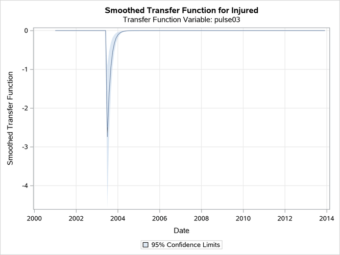
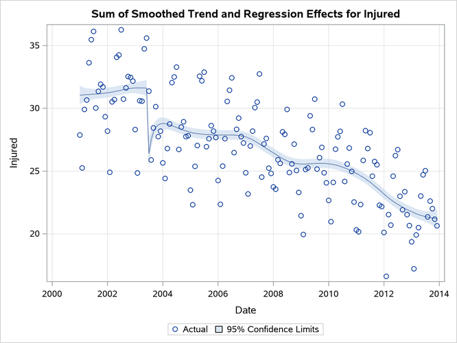
Output 41.10.3 shows the plot of smoothed estimate of the transfer function , and Output 41.10.4 shows the plot of the estimate of the trend plus the total effect of the July 2003 intervention.
Output 41.10.3: Decaying Part of the July 2003 Intervention Effect (Smoothed Estimate of )
Output 41.10.4: Smoothed Estimate of 
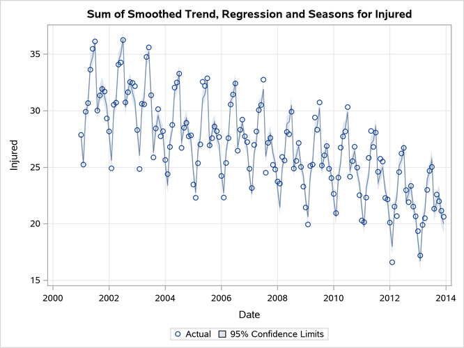
Finally, the Output 41.10.5 shows the plot of the overall model fit.
Output 41.10.5: Sum of All Model Terms Except the Irregular