UCM Procedure
Example 41.9 Extracting A Business Cycle
(View the complete code for this example.)
The data set (not shown) gdp in this example has two variables: date dates the observations, and lgdp contains the quarterly readings of the US real GDP (in log scale). Pelagatti (2015, Example 3.3, Example 8.2) uses this quarterly time series (lgdp) to illustrate how you can adjust the smoothness of the estimated cycle by changing the order of the cycle in a trend-cycle decomposition,

where  is an integrated random walk trend,
  is a cycle component, and
  is an irregular component.
The following statements fit the model  , where the cycle component has an order of 1 (default):
proc ucm data=gdp;
    where year(date) >= 1970;
    id date interval=quarter;
    model lgdp;
    irregular;
    level variance=0 noest plot=smooth;
    slope;
    cycle plot=smooth;
    estimate plot=panel;
    forecast plot=decomp outfor=for1;
run;
The following statements fit the same model, except that the cycle order is 2. Similarly, a model with a cycle order of 4 is also fit (not shown).
proc ucm data=gdp;
    where year(date) >= 1970;
    id date interval=quarter;
    model lgdp;
    irregular;
    level variance=0 noest plot=smooth;
    slope;
    cycle order=2 plot=smooth;
    estimate plot=panel;
    forecast plot=decomp outfor=for2;
run;
Output 41.9.1 summarizes the features of the estimated cycles of different orders. The estimated periods of the first-order and second-order cycles, 31.59 and 45.18, are reasonable. However, the period of the fourth-order cycle seems quite unreasonable. Fortunately, Pelagatti (2015, Example 8.2) mentions that cycles of order 3 or higher are rarely needed when you are working with real economic series. Although they are not the same, the parameter estimates that the UCM procedure produces are reasonably close to those reported in Pelagatti (2015, Example 8.2).
Output 41.9.1: Cycles of Orders 1, 2, and 4: Summary
| order | period | Frequency | Rho | ErrorVar |
|---|---|---|---|---|
| 1 | 31.59294 | 0.19888 | 0.94371 | 0.00004873 |
| 2 | 45.18259 | 0.13906 | 0.76177 | 0.00000956 |
| 4 | 38878 | 0.00016161 | 0.52055 | 0.00000856 |
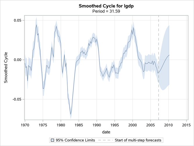
Output 41.9.2 shows the plot of the first-order cycle, Output 41.9.3 shows the plot of the second-order cycle, and Output 41.9.4 shows the plot of the fourth-order cycle. You can see that although the overall form of the estimated cycle remains the same, the smoothness of the plot of the estimated cycle increases with the order.
Output 41.9.2: Estimated Cycle: Order = 1
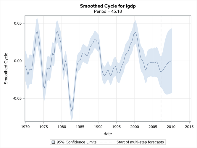
Output 41.9.3: Estimated Cycle: Order = 2
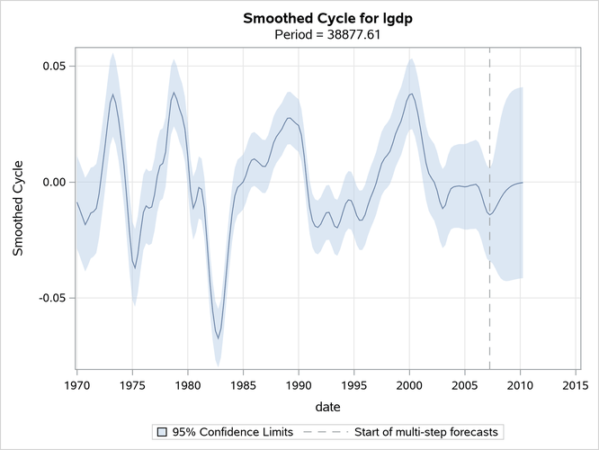
Output 41.9.4: Estimated Cycle: Order = 4
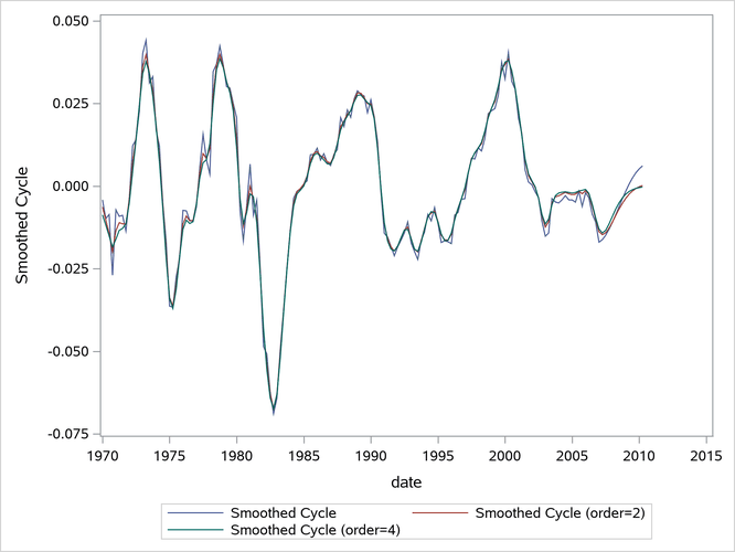
Output 41.9.5 shows the three cycle estimates in the same plot. It shows that the estimates don’t differ very much.
Output 41.9.5: Estimated Cycles of Orders 1, 2, and 4