SSM Procedure
Example 33.16 Temporal Distribution: Estimating Monthly GDP
(View the complete code for this example.)
This example is based on a case study described in Pelagatti (2015, chap. 9, Example 9.2). The case study shows how you can estimate the monthly GDP (gross domestic product) for the United States by temporally distributing the quarterly GDP time series, which is readily available. The temporal distribution process is based on a bivariate model that relates two variables, the quarterly GDP and the monthly industrial production index (both for the United States). Assuming that t denotes the monthly time index,  denotes the monthly industrial production index series, and
  denotes the quarterly GDP series that is organized as a monthly series (by setting the GDP numbers to missing for the months when they are not published), the case study uses the following model,

where
 is the unobserved monthly GDP series (which is to be estimated)
  is a bivariate trend component that follows an integrated random walk
  is a bivariate cycle component
  is a bivariate white noise component
As explained in the section Temporal Distribution, it is easy to fit this model by using the SSM procedure. As a first step, a data set, Useco, is created that organizes the monthly industrial production index and the quarterly GDP as monthly series. Specifically, Useco contains four variables: date dates the observations, indpro contains the monthly industrial production index, gdp contains the quarterly GDP, and startQ is a dummy variable that indicates the start of the quarter. This data set is essentially the same as the one that is used in the case study, except that, to improve the computational stability, gdp is scaled by 100. This data set has one peculiarity that is not mentioned in the case study: the GDP reporting pattern appears to have changed a few times over the years (October 1969, May 1992, and December 2014). The dummy variable, startQ, which indicates the start of the aggregation interval, is appropriately modified to take these changes into account. Output 33.16.1 shows the first few rows of Useco.
Output 33.16.1: First Few Rows of Useco
| date | startQ | gdp | indpro |
|---|---|---|---|
| 01JAN47 | 1 | . | 13.6351 |
| 01FEB47 | 0 | . | 13.7156 |
| 01MAR47 | 0 | 19.3447 | 13.7962 |
| 01APR47 | 1 | . | 13.6888 |
| 01MAY47 | 0 | . | 13.7425 |
| 01JUN47 | 0 | 19.3228 | 13.7425 |
| 01JUL47 | 1 | . | 13.6619 |
| 01AUG47 | 0 | . | 13.7425 |
The following statements show you how to specify the bivariate model for indpro and gdp:
 proc ssm data=useco opt(maxiter=100);
    id date interval=month;
   /* Bivariate integrated random walk */
   state irwState(2) type=ll(slopecov(g));
   comp irwInd = irwState[1];
   comp irwGdp = irwState[2];
   /* Bivariate cycle */
   state cycle(2) type=cycle cov(g);
   comp cycInd = cycle[1];
   comp cycGdp = cycle[2];
   /* Bivariate white noise */
   state noise(2) type=wn cov(g);
   comp noiseInd = noise[1];
   comp noiseGdp = noise[2];
   /* Observation equations */
   model indpro = irwInd cycInd noiseInd;
   model gdp = irwGdp cycGdp noiseGdp / distribute(start=startQ);
   /* Components for output */
   eval trendCycGdp = irwGdp + cycGdp;
   eval trendCycInd = irwInd + cycInd;
   eval monthlyGdp = irwGdp + cycGdp + noiseGdp;
   /* Output data set */
   output out=forGdp pdv press;
 run;
Here are a few comments about this program:
The first STATE statement specifies
irwStateas a bivariate trend that follows an integrated random walk (which is a local linear trend without the disturbance term in the level equation);irwStatecorresponds to . The trend components in the models for
 indproandgdpare specified in the two COMP statements that follow:irwIndandirwGdpcorrespond to and
and  , respectively.
 Similarly, the second STATE statement and the two COMP statements that follow it define
cycIndandcycGdpas the two cycle components ( and
and  ) in the model.
 The noise components,
noiseIndandnoiseGdp, which correspond to and
and  , respectively, are also defined in the same way.
 -
The MODEL statement for
indprocorresponds to the equation . On the other hand, the DISTRIBUTE(START=startQ) option in the MODEL statement of
 gdpcausesgdpto be modeled as an aggregated version of the unobserved monthly GDP series (): 
After the model specification is complete, EVAL statements are used to define some useful linear combinations of the components that are part of the model specification—for example,
monthlyGdp(which is defined as a sum ofirwGdp,cycGdp, andnoiseGdp) corresponds to the unobserved monthly GDP (). The SSM procedure outputs the estimates of these components to the data set that is specified in the OUT= option in the OUTPUT statement.
The parameter estimates in Output 33.16.2 are similar to (but not the same as) the parameter estimates reported in the case study. In particular, the estimates of the parameters of the cycle component—for example, the damping factor (Rho = 0.99228) and the period (293.32178)—are reasonably close.
Output 33.16.2: Estimated Model Parameters
| Model Parameter Estimates | |||||
|---|---|---|---|---|---|
| Component | Type | Parameter | Estimate | Standard Error |
t Value |
| irwState | Slope Disturbance Covari | RootCov[1, 1] | 0.10652 | 0.013572 | 7.85 |
| irwState | Slope Disturbance Covari | RootCov[2, 1] | 0.02060 | 0.002921 | 7.05 |
| irwState | Slope Disturbance Covari | RootCov[2, 2] | 0.00128 | 0.000507 | 2.52 |
| cycle | Damping Factor | Rho | 0.99228 | 0.004598 | 215.80 |
| cycle | Cycle Period | Period | 293.32178 | 94.269721 | 3.11 |
| cycle | Disturbance Covariance | RootCov[1, 1] | 0.32777 | 0.028788 | 11.39 |
| cycle | Disturbance Covariance | RootCov[2, 1] | 0.04196 | 0.013560 | 3.09 |
| cycle | Disturbance Covariance | RootCov[2, 2] | 0.06074 | 0.007665 | 7.92 |
| noise | Disturbance Covariance | RootCov[1, 1] | 0.08617 | 0.038876 | 2.22 |
| noise | Disturbance Covariance | RootCov[2, 1] | -0.12117 | 0.094158 | -1.29 |
| noise | Disturbance Covariance | RootCov[2, 2] | 0.03707 | 0.322549 | 0.11 |
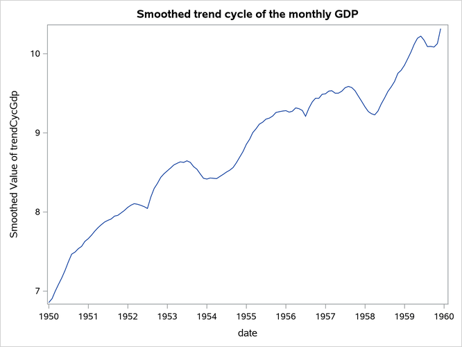
Figure 23 shows the plot of the estimated monthly GDP, and Figure 24 shows the plot of the estimate of monthly trend-cycle estimate ( ) for GDP.
Figure 23: Estimate of Monthly GDP
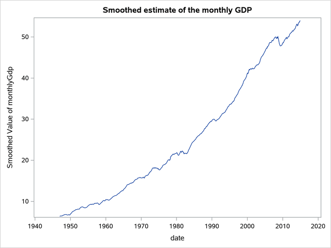
Figure 24: Smoothed Trend-Cycle Component of Monthly GDP (1950 to 1960)