SSM Procedure
Example 33.15 Longitudinal Data: Lung Function Analysis
(View the complete code for this example.)
The data for this example, which consist of 209 measurements of the lung function of an asthma patient, are analyzed in Wang (2013). The time series is measured mostly at two-hour time intervals but with irregular gaps. Wang (2013) fit a fourth-order continuous-time autoregressive model, CAR(4), to these data. The analysis results in a decomposition of the observed time series in three components:
a slowly varying trend pattern, which appears to have a slight downward drift
a diurnal component—a periodic pattern with a period of 24 hours
a residual component
As shown in Wang (2013), the continuous-time autoregressive models can be formulated as state space models. However, in general, the form of such SSMs is quite complex. Consequently, specifying such a model by using the current SSM procedure syntax is impractical. On the other hand, you can analyze these types of longitudinal data by using continuous-time structural models, which are easy to specify in the SSM procedure. In this example, the lung function measurements, y, are modeled as

where  is a simple linear time trend,
  is a continuous-time stochastic cycle, and
  is a Gaussian white noise sequence. Replacing the linear time trend with a more general time trend, such as a spline smoother, does not seem to change the fit, because the estimated smoothing spline turns out to be almost perfectly linear.
The following statements show you how to specify this model in the SSM procedure:
proc ssm data=asth;
   id time;
   state s1(1) type=cycle(CT) cov(g);
   comp c1 = s1[1];
   intercept = 1;
   irregular wn;
   model y= intercept time c1 wn;
   output out=for1 press;
   eval pattern=intercept+time+c1;
run;
The continuous-time stochastic cycle, named c1, is defined by a pair of STATE and COMPONENT statements. The STATE statement defines s1 as a state subsection that is associated with a univariate, continuous-time cycle (signified by the use of type=cycle(CT)). The COMPONENT statement defines c1 as its first element.
Output 33.15.1: Linear Time Trend: Estimates of Intercept and Slope
| Regression Parameter Estimates | |||||
|---|---|---|---|---|---|
| Response Variable | Regression Variable | Estimate | Standard Error |
t Value | Pr > |t| |
| y | intercept | 502.1637 | 3.50470 | 143.28 | <.0001 |
| y | time | -0.0201 | 0.00918 | -2.19 | 0.0286 |
Output 33.15.1 shows the estimated intercept and slope of the time trend. The estimated slope (only marginally significant) is negative, which is consistent with the overall downward drift.
Output 33.15.2: Estimated Stochastic Cycle:
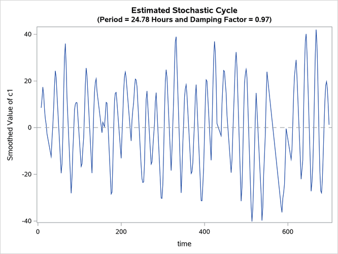
Output 33.15.2 shows the plot of the estimated cycle component, which has a period of 24.78 hours and a damping factor of 0.97. That is, it is a nearly persistent diurnal cycle.
Output 33.15.3: Estimated Pattern: 
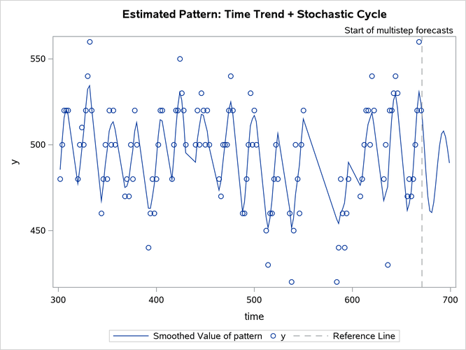
Output 33.15.3 shows the fit of the de-noised y values ( ). To reduce the clutter, only the second half of the data are plotted. The fit appears to be quite reasonable.