Shared Concepts
Splines and Spline Bases
This section provides details about how the spline parameter constructs spline bases. A spline function is a piecewise polynomial function in which the individual polynomials have the same degree and connect smoothly at join points whose abscissa values, called knots, are prespecified. You can use spline functions to fit curves to a wide variety of data.
A spline of degree 0 is a step function with steps located at the knots. A spline of degree 1 is a piecewise linear function where the lines connect at the knots. A spline of degree 2 is a piecewise quadratic curve whose values and slopes coincide at the knots. A spline of degree 3 is a piecewise cubic curve whose values, slopes, and curvature coincide at the knots. Visually, a cubic spline is a smooth curve, and it is the most commonly used spline when a smooth fit is desired. Note that when no knots are used, splines of degree d are simply polynomials of degree d.
More formally, suppose you specify knots  . Then a spline of degree
  is a function
  with d–1 continuous derivatives such that

where each  is a polynomial of degree d. The requirement that has d – 1 continuous derivatives is satisfied by requiring that the function values and all derivatives up to order d – 1 of the adjacent polynomials at each knot match.
A counting argument yields the number of parameters that define a spline with n knots. There are n + 1 polynomials of degree d, producing  coefficients. However, there are d restrictions at each of the n knots, so the number of free parameters is
  = n + d + 1. In mathematical terminology this says that the dimension of the vector space of splines of degree d on n distinct knots is n + d + 1. If you have n + d + 1 basis vectors, then you can fit a curve to your data by regressing your dependent variable by using this basis for the corresponding design matrix columns. In this context, such a spline is known as a regression spline. The
 spline parameter provides a simple mechanism for obtaining such a basis.
If you remove the restriction that the knots of a spline must be distinct and allow repeated knots, then you can obtain functions that have less smoothness and even discontinuities at the repeated knot location. For a spline of degree d and a repeated knot that has multiplicity  , the piecewise polynomials that join such a knot are required to have only d – m matching derivatives. Note that this increases the number of free parameters by m – 1 but also decreases the number of distinct knots by m – 1. Hence the dimension of the vector space of splines of degree d with n knots is still n + d + 1, provided that any repeated knot has a multiplicity less than or equal to d.
The spline parameter supports the commonly used truncated power function basis and B-spline basis. With exact arithmetic and by using the complete basis, you obtain the same fit with either of these bases. The following subsections provide details about constructing spline bases for the space of splines of degree d with n knots that satisfies  .
.
Truncated Power Function Basis
A truncated power function for a knot  is a function defined by

Figure 1 shows such functions for d = 1 and d = 3 with a knot at x = 1.
Figure 1: Truncated Power Functions with Knot at x = 1
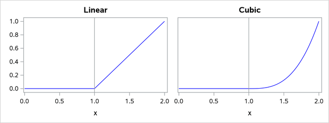
The name is derived from the fact that these functions are shifted power functions that are truncated to 0 to the left of the knot. These functions are piecewise polynomial functions that have two pieces whose function values and derivatives of all orders up to d–1 are 0 at the defining knot. Hence these functions are splines of degree d. It is easy to see that these n functions are linearly independent. However, they do not form a basis, because such a basis requires n+d–1 functions. The usual way to add d+1 additional basis functions is to use the polynomials  . These d+1 functions together with the n truncated power functions
  form the truncated power basis.
Note that each time a knot is repeated, the associated exponent used in the corresponding basis function is reduced by 1. For example, for splines of degree d with three repeated knots  , the corresponding basis functions are
  ,
,  , and
, and  . Provided that the multiplicity of each repeated knot is less than or equal to the degree, this construction continues to yield a basis for the associated space of splines.
The main advantage of the truncated power function basis is the simplicity of its construction and the ease of interpreting the parameters in a model that corresponds to these basis functions. However, there are two weaknesses when you use this basis for regression. These functions grow rapidly without bound as x increases, resulting in numerical precision problems when the x data span a wide range. Furthermore, many or even all of these basis functions can be nonzero when evaluated at some x value, resulting in a design matrix that has few zeros and precludes the use of sparse matrix technology to speed up computation. This weakness can be addressed by using a B-spline basis.
B-Spline Basis
A B-spline basis can be built by starting with a set of Haar basis functions, which are functions that are 1 between adjacent knots and 0 elsewhere, and then applying a simple linear recursion relationship d times, yielding the  needed basis functions. For the purpose of building the B-spline basis, the n prespecified knots are called internal knots. This construction requires d additional knots, known as boundary knots, to be positioned to the left of the internal knots, and
  boundary knots to be positioned to the right of the internal knots. The actual values of these boundary knots can be arbitrary. The
 spline parameter provides several methods for placing the necessary boundary knots, including the common method of using repeated values of the data extremes as the boundary knots. The boundary knot placement affects the precise form of the basis functions that are generated, but it does not affect the following two desirable properties:
The B-spline basis functions are nonzero over an interval that spans at most
 knots. This yields design matrix columns each of whose rows contain at most adjacent nonzero entries.
 The computation of the basis functions at any x value is numerically stable and does not require evaluating powers of this value.
The following figures show the B-spline bases that are defined on  with four equally spaced internal knots at 0.2, 0.4, 0.6, and 0.8.
Figure 2 shows a linear B-spline basis. This basis consists of six functions, each of which is nonzero over an interval that spans at most three knots.
Figure 2: Linear B-Spline Basis with Four Equally Spaced Interior Knots
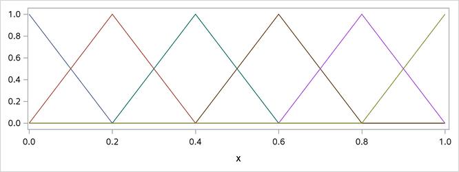
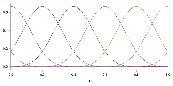
Figure 3 shows a cubic B-spline basis where the necessary boundary knots are positioned at x = 0 and x = 1. This basis consists of eight functions, each of which is nonzero over an interval that spans at most five knots.
Figure 3: Cubic B-Spline Basis with Four Equally Spaced Interior Knots
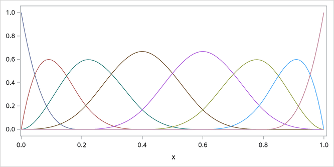
Figure 4 shows a different cubic B-spline basis where the necessary left-side boundary knots are positioned at –0.6, –0.4, –0.2, and 0. The right-side boundary knots are positioned at 1, 1.2, 1.4, and 1.6. As in the basis shown in Figure 3, this basis consists of eight functions, each of which is nonzero over an interval that spans at most five knots. The different positioning of the boundary knots has merely changed the shape of the individual basis functions.
Figure 4: Cubic B-Spline Basis with Equally Spaced Boundary and Interior Knots
For more information about this construction, see Hastie, Tibshirani, and Friedman (2001).
Natural Cubic Spline Basis
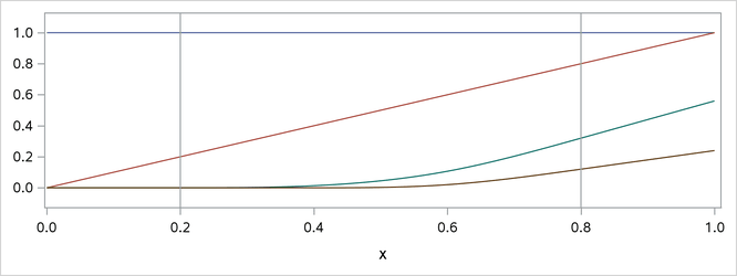
Natural cubic splines are cubic splines with the additional restriction that the splines are required to be linear beyond the extreme knots. Some authors prefer the terminology "restricted cubic splines" to "natural cubic splines." The space of unrestricted cubic splines on n knots has the dimension  . Imposing the restrictions that the cubic polynomials beyond the first and last knot reduce to linear polynomials reduces the number of degrees of freedom by 4, so a basis for the natural cubic splines consists of n functions. Starting from the truncated power function basis for the unrestricted cubic splines, you can obtain a reduced basis by imposing linearity constraints. For more information about this construction, see Hastie, Tibshirani, and Friedman (2001). Figure 5 shows this natural cubic spline basis defined on with four equally spaced internal knots at 0.2, 0.4, 0.6, and 0.8. This basis consists of four basis functions that are all linear beyond the extreme knots at 0.2 and 0.8.
Figure 5: Natural Cubic Spline Basis with Four Equally Spaced Knots